News
Extracting and Enriching OBIS Data with R
22 November 2016
- Introduction and Rationale
- Starting point, journey, and destination
- Taxonomy
- Getting occurrences
- Understanding occurrence records
- Enriching OBIS data
- Adding geography
- Coda
Introduction and Rationale
Programmatic access to biodiversity data is revolutionising large-scale, reproducible biodiversity research. In this series of tutorials we show how OBIS data can be accessed programmatically from within the Open Source statistical computing environment R. This exposes OBIS data to the full range of manipulations, visualisations, and statistical analyses provided by R. It also makes it possible to link and enrich OBIS data, combining it with other environmental, geographic, and biological data sets to better understand the distribution and dynamics of marine biodiversity. The examples we provide here constitute what we consider to be among the most common desired use cases of OBIS data, and they depend upon the considerable efforts of many in the R community who have contributed the useful packages which we have used. In particular, ROpenSci provides a wide range of open tools for open science, and our work has benefited greatly from working with and learning from them. Our hope is that other users will build on these examples, adapting and improving them to fit a range of research and policy scenarios.
Disclaimer: In all of the examples used here, data taken as is. Where possible we have alerted users to possible quality control issues but we cannot take responsibility for errors in the data. The code provides example implementations of the various use cases we envisage, but these will certainly not be the only ways to implement these methods, and may not be the most efficient or robust. Our code lives on GitHub here and we welcome suggestions for how to improve it.
The examples we provide build on the work of others, and use a large number of existing R packages. You will need to ensure that all of these (and their dependencies) are installed in order for the code in these tutorials to run. Most can be installed from CRAN in the standard manner, e.g. install.packages("package_name") but some are development versions which need to be installed from GitHub, for which you will need the devtools library installed (install.packages("devtools") if you need).
The packages we use development versions for need to be installed like this:
devtools::install_github("ropenscilabs/mregions")
devtools::install_github("iobis/robis")
devtools::install_github("ropensci/taxizesoap")
If you have problems installing taxizesoap see https://github.com/ropensci/taxizesoap. Once all packages are installed, load them:
library(taxizesoap)
library(robis)
library(ggmap)
library(dplyr)
library(ncdf4)
library(raster)
library(stringr)
library(readr)
library(pryr)
library(marmap)
library(lubridate)
library(broom)
library(mregions)
library(rgeos)
All data for this tutorial can be at https://github.com/iobis/training/tree/master/sorbycollection.
Starting point, journey, and destination
We choose to start with a list of taxonomic names of unknown quality. In our experience this is a common situation: you may have obtained a dataset from a collaborator, or from the literature, which documents some characteristics of a number of taxa, and you wish to tidy up this dataset and enrich it with some occurrence data. The taxon list we have chosen is one very local to us in landlocked Sheffield. On the wall in the Department of Animal and Plant Sciences at the University of Sheffield is a display case that is all too easy to walk past - some of us have been walking past it every day for years.

Light it up and examine the specimens though and they are revealed to be spectacular:

This collection was created by the 19th Century Sheffield microscopist, geologist, and naturalist Henry Clifton Sorby, using a technique for mounting entire specimens that he perfected - and one which proved so complex and laborious that it was not widely taken up, despite the beautiful results. The 80 specimens in the collection provide a useful test-case for modern biodiversity computational methods, as there is considerable taxonomic breadth (including fish as well as numerous invertebrate groups), but the names recorded are of inconsistent taxonomic rank, and - having been recorded well over 100 years ago - many are almost certainly no longer current.
The first stage of our journey then - after transcribing the names into a spreadsheet - is to check their taxonomy. Once we are confident in the names, and have restricted the dataset to a suitable taxonomic rank (species, here), we can start to examine occurrences as recorded in OBIS. Once we have done this, for individual species and for groups of species, we can start to enrich the basic occurrence data in various ways. In particular, we show how to match the occurrences to various environmental layers, including depth and climate. And we show how to perform more sophisticated geographic searches using georeferenced boundaries and regions.
Taxonomy
OBIS uses the WoRMS standard taxonomy. This means that names within OBIS’s realisation of the WoRMS Aphia database will be matched correctly - that is, occurrence records returned for an accepted taxonomic name will include records for unaccepted synonyms, and unaccepted names will be amalgamated to the current accepted name. However, it is often worthwhile to check your taxonomy in advance, especially if you are working with large sets of taxa (as macroecologists frequently are), or with unusual sets of names, such as the Sorby Collection. This will help to identify any potential problems or ambiguities, and also gives more flexibility for identifying and dealing with minor typos and misspellings. WoRMS provides options for matching relatively small lists of taxa (<1500 rows) via its website, with larger matches possible via the LifeWatch taxonomic backbone. For large and/or complex lists of taxa, for instance if you have little confidence in the names supplied, then working via WoRMS or LifeWatch in this way is probably a good idea. Certainly in our experience any sufficiently long list of taxa is going to require a certain amount of user interaction and informed or expert judgement in order to arrive at an acceptable taxonomic match. However, it is possible to rapidly match names to WoRMS by calling the WoRMS web services directly from within R, using the taxizesoap package. This provides much of the WoRMS taxon matching functionality, for instance fuzzy (or approximate) name matching is possible. This can provide a convenient, scripted way of generating a taxonomically robust dataset, and we demonstrate its use here.
First, read in a species list - here, the Sorby collection list, data available here. Note this uses the read_csv function from the readr package, which has some speed and parsing advantages over the base read.csv function. read_csv2 is appropriate if you are dealing with a csv from a country which uses ‘,’ as a decimal separator. This assumes that the sorby_collection data is in a subfolder data within your working directory:
sorby_coll <- read_csv("data/sorby_collection.csv")
Have quick look at the data - should be a single variable, taxon_name:
glimpse(sorby_coll)
## Observations: 50
## Variables: 1
## $ taxon_name <chr> "Actinoloba dianthus", "Alloteuthis media", "Aphrod...
Check taxonomy of a single taxon
Select the first species, Actinoloba dianthus:
my_sp <- sorby_coll$taxon_name[1]
Get AphiaID for this species. Here we set accepted = FALSE so that we are not restricted to accepted IDs (for instance, with accepted = TRUE no ID would be found for Actinoloba dianthus):
my_sp_aphia <- get_wormsid(searchterm = my_sp, accepted = FALSE)
##
## Retrieving data for taxon 'Actinoloba dianthus'
The full WoRMS record for this species can then be obtained from the ID as:
my_sp_taxo <- worms_records(ids = my_sp_aphia, marine_only = TRUE)
Note that you can choose whether to restrict the search to species classified as marine by WoRMS by setting the marine_only argument.
Use glimpse() for a quick overview of the returned dataframe:
glimpse(my_sp_taxo)
## Observations: 1
## Variables: 26
## $ inputid         <chr> "742385"
## $ AphiaID         <chr> "742385"
## $ url             <chr> "http://www.marinespecies.org/aphia.php?p=taxd...
## $ scientificname  <chr> "Actinoloba dianthus"
## $ authority       <chr> "de Blainville, 1830"
## $ rank            <chr> "Species"
## $ status          <chr> "unaccepted"
## $ unacceptreason  <chr> NA
## $ valid_AphiaID   <chr> "100982"
## $ valid_name      <chr> "Metridium senile"
## $ valid_authority <chr> "(Linnaeus, 1761)"
## $ kingdom         <chr> "Animalia"
## $ phylum          <chr> "Cnidaria"
## $ class           <chr> "Anthozoa"
## $ order           <chr> "Actiniaria"
## $ family          <chr> "Actinostolidae"
## $ genus           <chr> "Actinoloba"
## $ citation        <chr> "Fautin, D. (2013). Actinoloba dianthus de Bla...
## $ lsid            <chr> "urn:lsid:marinespecies.org:taxname:742385"
## $ isMarine        <chr> "1"
## $ isBrackish      <chr> NA
## $ isFreshwater    <chr> NA
## $ isTerrestrial   <chr> NA
## $ isExtinct       <chr> NA
## $ match_type      <chr> "exact"
## $ modified        <chr> "2013-10-04T10:33:40Z"
You can see from status that this name / ID is unaccepted; the valid_name is Metridium senile. You get the taxonomic hierarchy for this accepted name, and some habitat information (1 in isMarine shows that it is a marine species).
Check a list of taxa
More frequently you are likely to check want to check a list of taxa. To do that, simply pass the full list to the above functions. This will take a few seconds to run through the whole list. To avoid multiple calls for the same name, you should ensure your list contains each unique taxon name only once. In this example each name does only appear once in the sorby_coll, i.e.:
identical(length(unique(sorby_coll$taxon_name)), length(sorby_coll$taxon_name))
## [1] TRUE
If that is not the case, create a taxon list like this:
my_taxa <- unique(sorby_coll$taxon_name)
Then get AphiaIDs (this takes me ~20s to run):
system.time(
  all_spp_aphia <- get_wormsid(searchterm = my_taxa, accepted = FALSE)
)
##    user  system elapsed
##  12.928   0.249  21.526
You can check how many names were able to be linked to an AphiaID:
table(attr(all_spp_aphia, "match"))
##
##     found not found
##        47         3
So, all but three names were effectively matched. We will return to the 3 missing ones below. For now, add the returned AphiaIDs into our original dataframe:
sorby_coll$aphia_id <- as.vector(all_spp_aphia)
Sometimes multiple IDs will match a search term. This is especially likely to be the case if you search for a general common name, such as ‘cod’ - for example:
aphia_eg <- get_wormsid(searchterm = "cod", searchtype = "common", accepted = FALSE)
##
## Retrieving data for taxon 'cod'
##
##    AphiaID                     target     status    rank valid_AphiaID
## 1   105836           Alopias vulpinus   accepted Species        105836
## 2   158939                 Anas acuta   accepted Species        158939
## 3   126486          Antimora rostrata   accepted Species        126486
## 4   272297        Arctogadus borisovi   accepted Species        272297
## 5   126432       Arctogadus glacialis   accepted Species        126432
## 6   126433           Boreogadus saida   accepted Species        126433
## 7   126433           Boreogadus saida   accepted Species        126433
## 8   279397        Bothrocara brunneum   accepted Species        279397
## 9   234593           Bothrocara molle   accepted Species        234593
## 10  279400        Bothrocara pusillum   accepted Species        279400
## 11  313426       Bothrocara remigerum unaccepted Species        234593
## 12  126431     Bregmaceros atlanticus   accepted Species        126431
## 13  272290    Bregmaceros bathymaster   accepted Species        272290
## 14  158924        Bregmaceros cantori   accepted Species        158924
## 15  272291         Bregmaceros houdei   accepted Species        272291
## 16  158925  Bregmaceros macclellandii unaccepted Species        217740
## 17  217742     Bregmaceros mcclelandi unaccepted Species        217740
## 18  125468            Bregmacerotidae   accepted  Family        125468
## 19  151407            Champsodontidae   accepted  Family        151407
## 20  234518            Channichthyidae   accepted  Family        234518
## 21  137071          Clangula hyemalis   accepted Species        137071
## 22  218135         Cociella crocodila unaccepted Species        398453
## 23  145079               Codium bursa   accepted Species        145079
## 24  344030         Crocodylus porosus   accepted Species        344030
## 25  280501  Derepodichthys alepidotus   accepted Species        280501
## 26  254537          Eleginus gracilis   accepted Species        254537
## 27  267012             Euclichthyidae   accepted  Family        267012
## 28  158964           Gadella imberbis   accepted Species        158964
## 29  125469                    Gadidae   accepted  Family        125469
## 30  254538        Gadus macrocephalus   accepted Species        254538
## 31  126436               Gadus morhua   accepted Species        126436
## 32  126436               Gadus morhua   accepted Species        126436
## 33  158926                 Gadus ogac   accepted Species        158926
## 34  234704 Gobionotothen gibberifrons   accepted Species        234704
## 35  276514         Gobiosoma robustum   accepted Species        276514
## 36  126489      Halargyreus johnsonii   accepted Species        126489
## 37  232053       Haliaeetus albicilla   accepted Species        232053
## 38  232053       Haliaeetus albicilla   accepted Species        232053
## 39  232053       Haliaeetus albicilla   accepted Species        232053
## 40  144483              Halimeda tuna   accepted Species        144483
## 41  254960           Inia geoffrensis   accepted Species        254960
## 42  158979       Laemonema barbatulum   accepted Species        158979
## 43  217733         Lepidion ensiferus   accepted Species        217733
## 44  126493             Lepidion eques   accepted Species        126493
## 45  234788 Lepidonotothen squamifrons   accepted Species        234788
## 46  126555        Lophius piscatorius   accepted Species        126555
## 47  126103                Lycenchelys   accepted   Genus        126103
## 48  402539      Lycenchelys crotalina unaccepted Species        254592
## 49  274067        Lycenchelys jordani   accepted Species        274067
## 50  159257       Lycenchelys paxillus   accepted Species        159257
##                    valid_name
## 1            Alopias vulpinus
## 2                  Anas acuta
## 3           Antimora rostrata
## 4         Arctogadus borisovi
## 5        Arctogadus glacialis
## 6            Boreogadus saida
## 7            Boreogadus saida
## 8         Bothrocara brunneum
## 9            Bothrocara molle
## 10        Bothrocara pusillum
## 11           Bothrocara molle
## 12     Bregmaceros atlanticus
## 13    Bregmaceros bathymaster
## 14        Bregmaceros cantori
## 15         Bregmaceros houdei
## 16    Bregmaceros mcclellandi
## 17    Bregmaceros mcclellandi
## 18            Bregmacerotidae
## 19            Champsodontidae
## 20            Channichthyidae
## 21          Clangula hyemalis
## 22        Cociella crocodilus
## 23               Codium bursa
## 24         Crocodylus porosus
## 25  Derepodichthys alepidotus
## 26          Eleginus gracilis
## 27             Euclichthyidae
## 28           Gadella imberbis
## 29                    Gadidae
## 30        Gadus macrocephalus
## 31               Gadus morhua
## 32               Gadus morhua
## 33                 Gadus ogac
## 34 Gobionotothen gibberifrons
## 35         Gobiosoma robustum
## 36      Halargyreus johnsonii
## 37       Haliaeetus albicilla
## 38       Haliaeetus albicilla
## 39       Haliaeetus albicilla
## 40              Halimeda tuna
## 41           Inia geoffrensis
## 42       Laemonema barbatulum
## 43         Lepidion ensiferus
## 44             Lepidion eques
## 45 Lepidonotothen squamifrons
## 46        Lophius piscatorius
## 47                Lycenchelys
## 48     Lycenchelys crotalinus
## 49        Lycenchelys jordani
## 50       Lycenchelys paxillus
##
## More than one WoRMS ID found for taxon 'cod'!
##
##             Enter rownumber of taxon (other inputs will return 'NA'):
##
## Returned 'NA'!
Here, by default you will be asked to select one from the options provided, in interactive mode. Here I might chose option 31, if I know I am interested in Atlantic Cod, Gadus morhua. If you are running through a large list of species this interactivity can be inconvenient. In that case, you can set ask = FALSE in which case the function returns NA as an Aphia ID, but records the fact that multiple matches were found in the match attribute, e.g.:
aphia_eg <- get_wormsid(searchterm = "cod", searchtype = "common", accepted = FALSE, ask = FALSE)
##
## Retrieving data for taxon 'cod'
attr(aphia_eg, "match")
## [1] "multi match"
These cases can then be dealt with individually by the user. Note that when multiple matches are found, only first 50 will be returned, so it really does pay to make your taxon list as precise as possible, and to search on scientific rather than common names, especially if you have a large number of taxa to work through. (It is possible to overcome the 50 limit by setting an offset in worms_records, e.g. to return names starting at the 50th, but this is not covered here).
This gets the full worms_records for each species for which an AphiaID was found:
all_spp_taxa <- tbl_df(worms_records(ids = sorby_coll$aphia_id, marine_only = TRUE))
glimpse(all_spp_taxa)
## Observations: 47
## Variables: 26
## $ inputid         <chr> "742385", "153134", "231869", "129868", "10371...
## $ AphiaID         <chr> "742385", "153134", "231869", "129868", "10371...
## $ url             <chr> "http://www.marinespecies.org/aphia.php?p=taxd...
## $ scientificname  <chr> "Actinoloba dianthus", "Alloteuthis media", "A...
## $ authority       <chr> "de Blainville, 1830", "(Linnaeus, 1758)", "(L...
## $ rank            <chr> "Species", "Species", "Species", "Species", "S...
## $ status          <chr> "unaccepted", "accepted", "unaccepted", "accep...
## $ unacceptreason  <chr> NA, NA, "lapsus calami", NA, NA, NA, NA, "orig...
## $ valid_AphiaID   <chr> "100982", "153134", "129840", "129868", "10371...
## $ valid_name      <chr> "Metridium senile", "Alloteuthis media", "Aphr...
## $ valid_authority <chr> "(Linnaeus, 1761)", "(Linnaeus, 1758)", "Linna...
## $ kingdom         <chr> "Animalia", "Animalia", "Animalia", "Animalia"...
## $ phylum          <chr> "Cnidaria", "Mollusca", "Annelida", "Annelida"...
## $ class           <chr> "Anthozoa", "Cephalopoda", "Polychaeta", "Poly...
## $ order           <chr> "Actiniaria", "Myopsida", "Phyllodocida", NA, ...
## $ family          <chr> "Actinostolidae", "Loliginidae", "Aphroditidae...
## $ genus           <chr> "Actinoloba", "Alloteuthis", "Aphrodite", "Are...
## $ citation        <chr> "Fautin, D. (2013). Actinoloba dianthus de Bla...
## $ lsid            <chr> "urn:lsid:marinespecies.org:taxname:742385", "...
## $ isMarine        <chr> "1", "1", "1", "1", "1", "1", "1", "1", "1", "...
## $ isBrackish      <chr> NA, NA, "0", "0", NA, "0", NA, NA, "0", NA, NA...
## $ isFreshwater    <chr> NA, NA, "0", "0", "0", "0", NA, "0", "0", NA, ...
## $ isTerrestrial   <chr> NA, NA, "0", "0", "0", "0", NA, "0", "0", NA, ...
## $ isExtinct       <chr> NA, NA, NA, "0", NA, "0", NA, NA, "0", NA, NA,...
## $ match_type      <chr> "exact", "exact", "exact", "exact", "exact", "...
## $ modified        <chr> "2013-10-04T10:33:40Z", "2008-03-12T16:15:40Z"...
To check those species for which no Aphia was found, we can set some arguments in worms_records to do a more exhaustive search. First, identify the species:
taxa_to_check <- my_taxa[attr(all_spp_aphia, "match") == "not found"]
First, looks for non-marine matches:
worms_records(scientific = taxa_to_check, marine_only = FALSE)
## data frame with 0 columns and 0 rows
This returns nothing. Then, allow fuzzy (approximate) matching on the names:
worms_records(scientific = taxa_to_check, fuzzy = TRUE)
##               inputid  nil type
## 1   Bidoplax digitata <NA> <NA>
## 2 Chrysaora isosceles <NA> <NA>
## 3     Nerine vulgaris <NA> <NA>
This also returns nothing. So we conclude that these names are not present in WoRMS - the reasons why could be the subject of further investigation, referring back to the Sorby collection and cross-checking with other taxonomic authorities and experts.
Add worms_records back into our original dataframe:
sorby_coll <- left_join(sorby_coll, all_spp_taxa, by = c("aphia_id" = "inputid"))
glimpse(sorby_coll)
## Observations: 50
## Variables: 27
## $ taxon_name      <chr> "Actinoloba dianthus", "Alloteuthis media", "A...
## $ aphia_id        <chr> "742385", "153134", "231869", "129868", "10371...
## $ AphiaID         <chr> "742385", "153134", "231869", "129868", "10371...
## $ url             <chr> "http://www.marinespecies.org/aphia.php?p=taxd...
## $ scientificname  <chr> "Actinoloba dianthus", "Alloteuthis media", "A...
## $ authority       <chr> "de Blainville, 1830", "(Linnaeus, 1758)", "(L...
## $ rank            <chr> "Species", "Species", "Species", "Species", "S...
## $ status          <chr> "unaccepted", "accepted", "unaccepted", "accep...
## $ unacceptreason  <chr> NA, NA, "lapsus calami", NA, NA, NA, NA, NA, "...
## $ valid_AphiaID   <chr> "100982", "153134", "129840", "129868", "10371...
## $ valid_name      <chr> "Metridium senile", "Alloteuthis media", "Aphr...
## $ valid_authority <chr> "(Linnaeus, 1761)", "(Linnaeus, 1758)", "Linna...
## $ kingdom         <chr> "Animalia", "Animalia", "Animalia", "Animalia"...
## $ phylum          <chr> "Cnidaria", "Mollusca", "Annelida", "Annelida"...
## $ class           <chr> "Anthozoa", "Cephalopoda", "Polychaeta", "Poly...
## $ order           <chr> "Actiniaria", "Myopsida", "Phyllodocida", NA, ...
## $ family          <chr> "Actinostolidae", "Loliginidae", "Aphroditidae...
## $ genus           <chr> "Actinoloba", "Alloteuthis", "Aphrodite", "Are...
## $ citation        <chr> "Fautin, D. (2013). Actinoloba dianthus de Bla...
## $ lsid            <chr> "urn:lsid:marinespecies.org:taxname:742385", "...
## $ isMarine        <chr> "1", "1", "1", "1", "1", "1", "1", NA, "1", "1...
## $ isBrackish      <chr> NA, NA, "0", "0", NA, "0", NA, NA, NA, "0", NA...
## $ isFreshwater    <chr> NA, NA, "0", "0", "0", "0", NA, NA, "0", "0", ...
## $ isTerrestrial   <chr> NA, NA, "0", "0", "0", "0", NA, NA, "0", "0", ...
## $ isExtinct       <chr> NA, NA, NA, "0", NA, "0", NA, NA, NA, "0", NA,...
## $ match_type      <chr> "exact", "exact", "exact", "exact", "exact", "...
## $ modified        <chr> "2013-10-04T10:33:40Z", "2008-03-12T16:15:40Z"...
Now, prior to querying OBIS, we might want to tidy up this dataset. For instance, we could strip out taxa for which we could not find a valid AphiaID or a valid name:
sorby_coll <- subset(sorby_coll, !is.na(valid_AphiaID) & !is.na(valid_name))
We might also want to restrict further analysis to a particular taxonomic rank. Let’s look at what ranks are present:
table(sorby_coll$rank)
##
##   Class  Family   Genus Species
##       2       1       4      38
For now we will work only on species:
sorby_coll <- subset(sorby_coll, rank == "Species")
NOTE: taxonomy is difficult, and resolving it tends to be messy, especially when large numbers of names are considered. For instance, the first species in our list is Actinoloba dianthus (ID 742385), which, when run through the process above, returns the ‘accepted’ ID 100982, for Metridium senile (Linnaeus, 1761). However, this in turn is actually unaccepted, and points to a different accepted ID (158251) and name, Metridium dianthus (Ellis, 1768):
worms_records(ids = "100982")
##   inputid AphiaID
## 1  100982  100982
##                                                             url
## 1 http://www.marinespecies.org/aphia.php?p=taxdetails&id=100982
##     scientificname        authority    rank     status unacceptreason
## 1 Metridium senile (Linnaeus, 1761) Species unaccepted           <NA>
##   valid_AphiaID         valid_name valid_authority  kingdom   phylum
## 1        158251 Metridium dianthus   (Ellis, 1768) Animalia Cnidaria
##      class      order      family     genus
## 1 Anthozoa Actiniaria Metridiidae Metridium
##                                                                                                                                                                                                                                          citation
## 1 Fautin, D. (2015). Metridium senile (Linnaeus, 1761). In: Fautin, Daphne G. (2013). Hexacorallians of the World. Accessed through:  World Register of Marine Species at http://marinespecies.org/aphia.php?p=taxdetails&id=100982 on 2016-09-09
##                                        lsid isMarine isBrackish
## 1 urn:lsid:marinespecies.org:taxname:100982        1       <NA>
##   isFreshwater isTerrestrial isExtinct match_type             modified
## 1         <NA>          <NA>      <NA>      exact 2015-10-13T12:34:41Z
To avoid (near)infinite recursion, we have stopped after one round of checking in WoRMS, but users may wish to run the above process more than once, or to randomly check some names in their lists, to ensure that they are confident in their results.
One further modification that may be useful is to add additional taxonomic levels beyond the standard ones returned by worms_records. For instance, ‘fish’ can be identified as a group using the non-standard Superclass = Pisces. This function simply returns a TRUE/FALSE flag telling you whether a given AphiaID belongs to Pisces or not:
get_pisces <- function(aphiaid){
  # get hierarchy for a given aphia ID
  if(exists("aphia_h")){rm(aphia_h)}
  pisces <- FALSE
  try(aphia_h <- worms_hierarchy(ids = aphiaid), silent = T)
  if(exists("aphia_h")){
    if("Pisces" %in% aphia_h$scientificname){
      pisces <- TRUE
    }
  }
  return(pisces)
}
Although it takes aphiaid as an input, it can easily be applied to scientific names by running, for instance:
get_pisces(get_wormsid("Gadus morhua", verbose = FALSE))
## [1] TRUE
We can add a pisces column to our dataset like this:
sorby_coll$pisces <- with(sorby_coll, sapply(valid_AphiaID, function(valid_AphiaID){get_pisces(valid_AphiaID)}))
This seems to have produced sensible results:
glimpse(subset(sorby_coll, pisces == TRUE))
## Observations: 5
## Variables: 28
## $ taxon_name      <chr> "Lipophrys pholis", "Merlangius merlangus", "P...
## $ aphia_id        <chr> "126768", "126438", "127143", "127160", "127387"
## $ AphiaID         <chr> "126768", "126438", "127143", "127160", "127387"
## $ url             <chr> "http://www.marinespecies.org/aphia.php?p=taxd...
## $ scientificname  <chr> "Lipophrys pholis", "Merlangius merlangus", "P...
## $ authority       <chr> "(Linnaeus, 1758)", "(Linnaeus, 1758)", "Linna...
## $ rank            <chr> "Species", "Species", "Species", "Species", "S...
## $ status          <chr> "accepted", "accepted", "accepted", "accepted"...
## $ unacceptreason  <chr> NA, NA, NA, NA, NA
## $ valid_AphiaID   <chr> "126768", "126438", "127143", "127160", "127387"
## $ valid_name      <chr> "Lipophrys pholis", "Merlangius merlangus", "P...
## $ valid_authority <chr> "(Linnaeus, 1758)", "(Linnaeus, 1758)", "Linna...
## $ kingdom         <chr> "Animalia", "Animalia", "Animalia", "Animalia"...
## $ phylum          <chr> "Chordata", "Chordata", "Chordata", "Chordata"...
## $ class           <chr> "Actinopteri", "Actinopteri", "Actinopteri", "...
## $ order           <chr> "Perciformes", "Gadiformes", "Pleuronectiforme...
## $ family          <chr> "Blenniidae", "Gadidae", "Pleuronectidae", "So...
## $ genus           <chr> "Lipophrys", "Merlangius", "Pleuronectes", "So...
## $ citation        <chr> "Bailly, N. (2008). Lipophrys pholis (Linnaeus...
## $ lsid            <chr> "urn:lsid:marinespecies.org:taxname:126768", "...
## $ isMarine        <chr> "1", "1", "1", "1", "1"
## $ isBrackish      <chr> "0", "0", "1", "1", "1"
## $ isFreshwater    <chr> "0", "0", "0", "0", "0"
## $ isTerrestrial   <chr> "0", "0", "0", "0", "0"
## $ isExtinct       <chr> NA, NA, NA, NA, NA
## $ match_type      <chr> "exact", "exact", "exact", "exact", "exact"
## $ modified        <chr> "2008-01-15T18:27:08Z", "2008-01-15T18:27:08Z"...
## $ pisces          <lgl> TRUE, TRUE, TRUE, TRUE, TRUE
We now have a species list with full validated WoRMS records for each, which we can now use to start to query OBIS.
Getting occurrences
Once you have your taxon name, or list of names, it is straightforward to extract their OBIS occurrences using the robis package. If you are confident that your original list of names is taxonomically correct, free of typos, etc. then you can search directly on them. However, as outlined above, we recommend some basic taxonomic checks which will then allow you to search directly either on AphiaIDs, or on confirmed valid species names. The latter has some benefits in terms of interpreting the output from a search. Once you have obtained a list of occurrences for a given taxon, you can very quickly produce a quick map. You can also obtain occurrences for whole lists of species, with the proviso that the returned data can rapidly become large, especially if all fields are returned (see Understanding occurrence records). Here we show how to obtain and map occurrence records for a single species, and then for a list of species.
Getting OBIS records for a single species
This is simply achieved using the robis::occurrence function. Note however that queries can take a while, especially if your species has a very large number of records. The first species in our dataset has a moderate number of records so is a good test case - it takes ~1 minute to run:
my_occs <- occurrence(scientificname = sorby_coll$valid_name[1])
This results in a tibble (a dataframe modified to display nicely on screen) with 7,267 rows - one for each record of Metridium senile - and 65 columns. This may seem like a lot of variables, but many of them are useful, as will be explained below. For now, we might want to get some basic summary information, for instance, what are the geographic limits of this set of occurrences? There are various ways to do this, here we will use the bbox function from the sp package:
bb_occs <- bbox(cbind(my_occs$decimalLongitude, my_occs$decimalLatitude))
bb_occs
##         min    max
## x -173.5000 145.57
## y  -48.3603  70.60
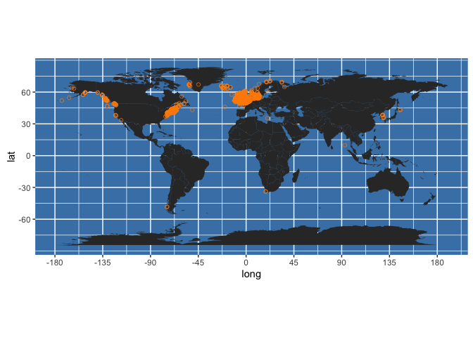
This shows that this species has been recorded very widely, from -173.5 to +145.57 degrees longitude and from -48.36 to +70.60 degrees latitude. We can quickly and roughly plot these data using ggmap functions. For a world map, use data from the maps package:
world <- map_data("world")
This creates a quick and dirty world map - playing around with the themes, aesthetics, and device dimensions is recommended!
worldmap <- ggplot(world, aes(x=long, y=lat)) +
  geom_polygon(aes(group=group)) +
  scale_y_continuous(breaks = (-2:2) * 30) +
  scale_x_continuous(breaks = (-4:4) * 45) +
  theme(panel.background = element_rect(fill = "steelblue")) +
  coord_equal()
Now add the occurrence points:
occ_map <- worldmap + geom_point(data = my_occs, aes(x = decimalLongitude, y = decimalLatitude),
                                 colour = "darkorange", shape = 21, alpha = 2/3)
occ_map
 You can change the projection using coord_map, for instance:
occ_map + coord_map("ortho")
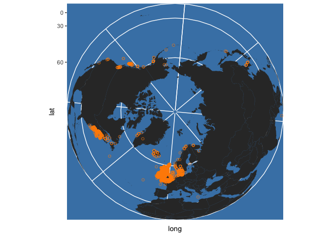
See ?coord_map for more details. Note that the code above does not treat the latitudes and longitudes obtained from OBIS as true spatial points with an associated projection. For more precise mapping this should be done. Projections are provided for some points, but not for many on this occasion - see:
table(my_occs$geodeticDatum)
##
## WGS84
##    10
Only 10 of the occurrences have associated projection details (here WGS84) - WGS84 is a sensible default though if you want to project the whole set of occurrences for more formal spatial analysis than we cover here. An alternative mapping approach, which doesn’t work well for global scale maps but can produce nice regional maps, is to get a basemap from google maps, here by feeding it your bounding box:
my_map <- get_map(
  location = bb_occs, maptype = "satellite"
)
Then add points to this base map like this:
ggmap(my_map) +
  geom_point(data = my_occs, aes(x = decimalLongitude, y = decimalLatitude),
             colour = "darkorange", shape = 21, alpha = 2/3)
## Warning: Removed 117 rows containing missing values (geom_point).
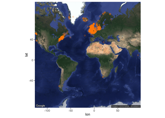
This will throw a warning about removing 117 rows which do not fit on this map. You can try playing around with the get_map function, in particular the zoom argument, to see if you can overcome this but it seems to be a limitation with global scale data (see here) - but the map should work fine if your set of occurrences is less geographically extensive.
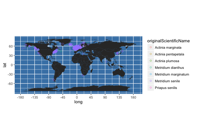
There are many options for modifying the map, for instance, you could colour code points by the original scientific name recorded (which OBIS has translated into the accepted name):
worldmap + geom_point(data = my_occs,
                      aes(x = decimalLongitude, y = decimalLatitude, colour = originalScientificName), shape = 21, alpha = 2/3)
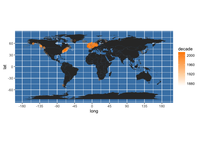
Or you could colour code by year collected. First, we can round yearcollected to give us decade collected:
my_occs$decade <- with(my_occs, 10*round(yearcollected/10, 0))
Then plot like this:
worldmap + geom_point(data = my_occs,
                      aes(x = decimalLongitude, y = decimalLatitude, colour = decade), shape = 21, alpha = 2/3) +
  scale_colour_gradient(low = "white", high = "darkorange")
The time taken to return occurrences scales with the number of occurrences, so beware that getting global occurrences for well-sampled species will take some time. To take an example from our dataset, the Dover sole Solea solea (Linnaeus, 1758) has a moderately large number of records (64781), which take approximately 2.5 minutes to obtain:
sole_occs <- occurrence(scientificname = "Solea solea")
The returned dataframe is also rather large:
object_size(sole_occs)
## 35.7 MB
So, if you anticipate returning large quantities of data from OBIS, it may make sense to limit the fields returned - for instance, you can drastically reduce the size of the data set (and the speed of the query) by returning only the first four fields (ID, lon, lat, and depth):
object_size(sole_occs[, 1:4])
## 1.81 MB
In addition, you can pre-filter the occurrences to be returned, e.g. by geographic region, or by other properties of the records, as outlined below.
Nonetheless, you can still easily produce maps with these large numbers of points:
bb_sole <- bbox(SpatialPoints(cbind(sole_occs$decimalLongitude, sole_occs$decimalLatitude)))
bb_sole
##                min     max
## coords.x1 -42.0288 151.639
## coords.x2 -33.0868  61.250
sole_map <- get_map(
  location = bb_sole, maptype = "satellite"
)

(sole_map <- ggmap(sole_map) +
  geom_point(data = sole_occs, aes(x = decimalLongitude, y = decimalLatitude),
             colour = "darkorange", shape = 21, alpha = 2/3)
)

Here is a more generic function to produce maps from data returned by robis::occurrence:
obis_map <- function(occ_dat, map_type = c("satellite", "world"), map_zoom = NULL, plotit = TRUE){

  bb_occ <- bbox(cbind(occ_dat$decimalLongitude, occ_dat$decimalLatitude))

  if(map_type == "satellite"){
    if(is.null(map_zoom)){
      base_map <- get_map(location = bb_occ, maptype = "satellite")
    } else {
      base_map <- get_map(location = bb_occ, maptype = "satellite", zoom = map_zoom)
    }
    obis_map <- ggmap(base_map)
  } else if(map_type == "world"){
    base_map <- map_data("world")
    obis_map <- ggplot(base_map, aes(x=long, y=lat)) +
      geom_polygon(aes(group=group)) +
      scale_y_continuous(breaks = (-2:2) * 30) +
      scale_x_continuous(breaks = (-4:4) * 45) +
      theme(panel.background = element_rect(fill = "steelblue")) +
      coord_equal()
  } else {
    stop("map_type must be one of 'satellite' or 'world'",
         call. = FALSE)
  }

  # Now add the occurrence points
  obis_map <- obis_map + geom_point(data = occ_dat, aes(x = decimalLongitude, y = decimalLatitude),
                                    colour = "darkorange", shape = 21, alpha = 2/3)

  if(plotit == T){print(obis_map)}

  return(obis_map)

}
Run it like this:
sole_map <- obis_map(sole_occs, map_type = "satellite")

Create the plot without plotting it:
sole_map <- obis_map(sole_occs, map_type = "satellite", plotit = FALSE)
If you do not have any prior knowledge about the likely number of OBIS records available for your taxa, and you wish to check before beginning potentially lengthy downloads, you can very rapidly (<0.1 second) get summary data for a given taxon, including the total number of OBIS records, using the taxa function. For sole, you get:
sole_summ <- checklist(scientificname = "Solea solea")
sole_summ$records
## [1] 64781
So this immediately alerts you to the fact that processing the individual records may be rather slow. You can run this function using scientific name or Aphia ID, and can run it for a list of taxa like this:
taxa_summ <- with(sorby_coll, sapply(valid_name, function(valid_name){checklist(scientificname = valid_name)}))
# equivalently for aphia ID (not run):
# taxa_summ <- with(sorby_coll, sapply(valid_AphiaID, function(valid_AphiaID){taxa(aphiaid = valid_AphiaID)}))
Note running the above over a list of taxa returns a list of data frames, one dataframe for each species. Processing these data frames is complicated slightly by the fact that different numbers of variables are returned for different species, depending on the metadata available for that species:
lengths(taxa_summ)
##     Metridium senile    Alloteuthis media   Aphrodita aculeata
##                   15                   15                   15
##     Arenicola marina   Ascidiella aspersa       Aurelia aurita
##                   14                   16                   15
## Botryllus schlosseri   Branchiomma bombyx      Carcinus maenas
##                   15                   15                   16
##   Ciona intestinalis
##                   16
##  [ reached getOption("max.print") -- omitted 28 entries ]
table(lengths(taxa_summ))
##
## 14 15 16 17
##  2 28  4  4
lapply(taxa_summ, names)
## $`Metridium senile`
##  [1] "id"        "valid_id"  "parent_id" "rank_name" "tname"
##  [6] "tauthor"   "worms_id"  "records"   "datasets"  "phylum"
##  [ reached getOption("max.print") -- omitted 5 entries ]
##
## $`Alloteuthis media`
##  [1] "id"        "valid_id"  "parent_id" "rank_name" "tname"
##  [6] "tauthor"   "worms_id"  "records"   "datasets"  "phylum"
##  [ reached getOption("max.print") -- omitted 5 entries ]
##
## $`Aphrodita aculeata`
##  [1] "id"        "valid_id"  "parent_id" "rank_name" "tname"
##  [6] "tauthor"   "worms_id"  "records"   "datasets"  "phylum"
##  [ reached getOption("max.print") -- omitted 5 entries ]
##
## $`Arenicola marina`
##  [1] "id"        "valid_id"  "parent_id" "rank_name" "tname"
##  [6] "tauthor"   "worms_id"  "records"   "datasets"  "phylum"
##  [ reached getOption("max.print") -- omitted 4 entries ]
##
## $`Ascidiella aspersa`
##  [1] "id"        "valid_id"  "parent_id" "rank_name" "tname"
##  [6] "tauthor"   "worms_id"  "gisd"      "records"   "datasets"
##  [ reached getOption("max.print") -- omitted 6 entries ]
##
## $`Aurelia aurita`
##  [1] "id"        "valid_id"  "parent_id" "rank_name" "tname"
##  [6] "tauthor"   "worms_id"  "records"   "datasets"  "phylum"
##  [ reached getOption("max.print") -- omitted 5 entries ]
##
## $`Botryllus schlosseri`
##  [1] "id"        "valid_id"  "parent_id" "rank_name" "tname"
##  [6] "tauthor"   "worms_id"  "records"   "datasets"  "phylum"
##  [ reached getOption("max.print") -- omitted 5 entries ]
##
## $`Branchiomma bombyx`
##  [1] "id"        "valid_id"  "parent_id" "rank_name" "tname"
##  [6] "tauthor"   "worms_id"  "records"   "datasets"  "phylum"
##  [ reached getOption("max.print") -- omitted 5 entries ]
##
## $`Carcinus maenas`
##  [1] "id"        "valid_id"  "parent_id" "rank_name" "tname"
##  [6] "tauthor"   "worms_id"  "gisd"      "records"   "datasets"
##  [ reached getOption("max.print") -- omitted 6 entries ]
##
## $`Ciona intestinalis`
##  [1] "id"        "valid_id"  "parent_id" "rank_name" "tname"
##  [6] "tauthor"   "worms_id"  "gisd"      "records"   "datasets"
##  [ reached getOption("max.print") -- omitted 6 entries ]
##
##  [ reached getOption("max.print") -- omitted 28 entries ]
For our purposes, we just want to extract one variable, ‘records’, the total number of OBIS records for each taxon. There is one further complication that we need to deal with before doing this: checklist will return data for taxonomic children of the taxon queried. For example, from our dataset:
eg_taxon <- checklist(scientificname = "Ciona intestinalis")
Returns 3 records, of different taxonomic ranks:
table(eg_taxon$rank_name)
##
##    Species Subspecies
##          1          2
The simplest option here is to sum the number of OBIS records across all children of each taxon:
obis_n <- tbl_df(data.frame(
  valid_name = names(taxa_summ),
  obis_n = unlist(lapply(taxa_summ, function(m) sum(m$records)))
))
This can then be joined back to our master dataframe:
sorby_coll <- left_join(sorby_coll, obis_n, by = "valid_name")
dplyr::select(sorby_coll, valid_name, obis_n)
## # A tibble: 38 × 2
##              valid_name obis_n
##                   <chr>  <int>
## 1      Metridium senile   7267
## 2     Alloteuthis media    374
## 3    Aphrodita aculeata   5177
## 4      Arenicola marina  13115
## 5    Ascidiella aspersa   5059
## 6        Aurelia aurita   3136
## 7  Botryllus schlosseri   9455
## 8    Branchiomma bombyx    446
## 9       Carcinus maenas  21313
## 10   Ciona intestinalis   5017
## # ... with 28 more rows
(Note the need to specify the package from which we want to run the select function here, as there is a select function in raster too. The package::function format is good practice whenever there might be ambiguity).
Have a look at the distribution of the number of OBIS records across taxa - easier on a log10 scale:
ggplot(sorby_coll, aes(x = obis_n)) + geom_histogram() + scale_x_log10()
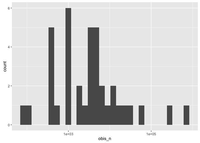
For the whole set of species in our list, there are about 1.25M records in OBIS:
sum(sorby_coll$obis_n)
## [1] 1248808
We will see below how to get similar summaries by geographic region, both for a pre-defined taxonomic list, and to generate a list for a region directly from OBIS.
First, let’s try running a full OBIS query over our complete list of species. Remember - this is going to return a dataframe with over 1M rows. To keep this more manageable in size, we will restrict the fields returned to the ‘essential’ variables of taxon name, lon and lat, depth, and year. Then get all OBIS records for all species - BE WARNED, this takes ~30 minutes to run:
allspp_obis <- with(sorby_coll, sapply(valid_name, function(valid_name){
  occurrence(scientificname = valid_name,
             fields = c("scientificName", "decimalLongitude", "decimalLatitude", "depth", "yearcollected"))}))
To convert the returned data into a neat dataframe:
allspp_obis <- bind_rows(apply(allspp_obis, 2, as.data.frame))
object_size(allspp_obis)
## 45 MB
This condition should be true:
identical(nrow(allspp_obis), sum(sorby_coll$obis_n))
## [1] TRUE
You can get some summary info here, such as the range in sample depths, as a histogram:
ggplot(allspp_obis, aes(x = depth)) + geom_histogram()
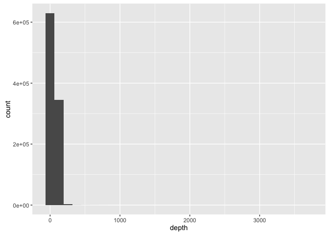
Or as quartiles:
quantile(allspp_obis$depth, 0:4/4, na.rm = T)
##   0%  25%  50%  75% 100%
##   -9   28   45   80 3678
This can be useful for quickly spotting unusual records - such as extreme depths (max here = 3678m), or possible missing value codes - 23689 records here have a depth value of -9, suggesting this has been used in some datasets as a missing value code:
sum(allspp_obis$depth == -9, na.rm = T)
## [1] 23689
We will consider how to address this further in the next section.
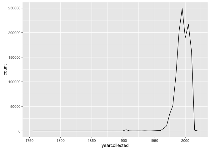
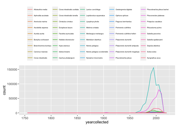
You might also want to look at number of records by year:
ggplot(allspp_obis, aes(x = yearcollected)) + geom_freqpoly(binwidth = 5)
Which you could split by species, either using colour:
ggplot(allspp_obis, aes(x = yearcollected, colour = scientificName)) + geom_freqpoly(binwidth = 5)+
  theme(legend.position = "top") +
  theme(legend.text = element_text(size = 5)) +
  theme(legend.title = element_blank())
Or as different facets:
ggplot(allspp_obis, aes(x = yearcollected)) + geom_freqpoly(binwidth = 5) +
  facet_wrap(~ scientificName, scales = "free_y")+
  theme(strip.text.x = element_text(size = 4)) +
  theme(axis.text.x = element_text(angle = 90, hjust = 1, size = 5))
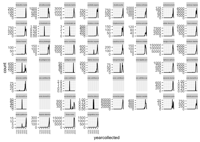
None of these plots are especially polished, but are intended to give some ideas that can be developed further.
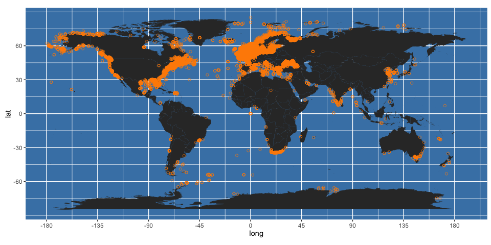
We can plot all of these records on a map (which will take a while to render, with >1.2M points):
worldmap + geom_point(data = allspp_obis,
                      aes(x = decimalLongitude, y = decimalLatitude), colour = "darkorange", shape = 21, alpha = 2/3)
It may be preferable in these cases to plot the data on a grid. Here, we create a 5x5 degree global grid:
global_grid <- raster(nrows = 180/5, ncol = 360/5, xmn = -180, xmx = 180, ymn = -90, ymx = 90)
Get the longitude and latitude of the OBIS records:
lonlat_sp <- cbind(x = allspp_obis$decimalLongitude, y = allspp_obis$decimalLatitude)
And sum these over the grid:
gridded_occs <- rasterize(x = lonlat_sp, y = global_grid, fun = "count")
To render these using ggplot, I’ve adapted some code from here. First, turn the gridded data back into a dataframe of points, and name the variables sensibly:
obis.p <- data.frame(rasterToPoints(gridded_occs))
names(obis.p) <- c("longitude", "latitude", "OBIS")
Then add these using geom_raster to the worldmap generated previously:
(worldmap + geom_raster(data = obis.p, aes(x = longitude, y = latitude, fill = OBIS)) +
  scale_fill_gradient(low = "white", high = "darkorange")
)
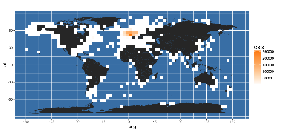
It may be better to display logged counts:
(gridded_obis <- worldmap + geom_raster(data = obis.p, aes(x = longitude, y = latitude, fill = log10(OBIS))) +
   scale_fill_gradient(low = "white", high = "darkorange")
)
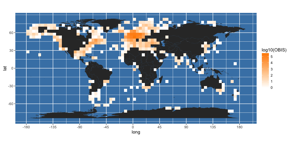
It is clear from this map that some points are falling on land. You can get a better idea of this by changing the transparency (alpha) value of the fill in the above plot:
worldmap + geom_raster(data = obis.p, aes(x = longitude, y = latitude, fill = log10(OBIS)), alpha = 2/3) +
  scale_fill_gradient(low = "white", high = "darkorange")
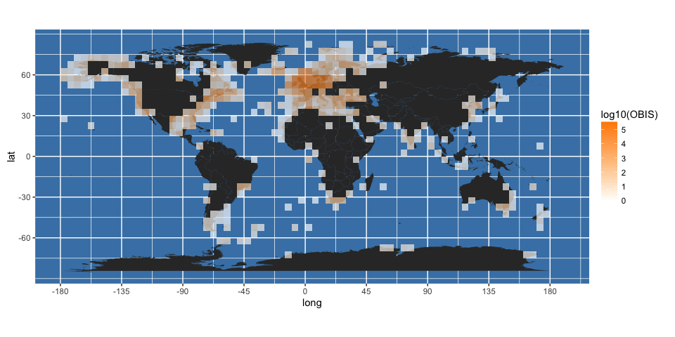
There are various reasons why this may be, ranging from an artifact of the 5-degree binning used, to the level of precision in the location data, to real errors. The next section explains how some additional data from OBIS can be used for initial quality control of returned data.
Understanding occurrence records
As macroecologists, we are typically interested in a relatively small set of variables when returning occurrence data from OBIS. These may reduce to simply taxon name, and the latitude and longitude of each record, perhaps supplemented by the date on which the occurrence was recorded, and the depth of sampling. However, using the methods above with default settings returns by default a dataframe with many columns, often 50 or more (the number varies with taxon). This might seem like overkill, and it may be tempting to restrict the fields that are returned, which can be simply implemented within R in various ways - here we demonstrate how to limit the fields returned from OBIS, and how to select only relevant columns from the returned data. But although this is sometimes going to be sensible (and certainly brings important memory savings when the returned set of occurrences is very large), it is worth understanding these different columns before discarding them. Here we investigate some of the fields returned, and show how to filter your results based on values of any of these, individually or in combination.
Examining OBIS records in more detail
glimpse(sole_occs)
## Observations: 64,781
## Variables: 54
## $ id                            <int> 343136975, 345256421, 345256359,...
## $ decimalLongitude              <dbl> -8.6240000, 6.4970000, 3.7851667...
## $ decimalLatitude               <dbl> 54.61800, 54.79467, 52.47767, 50...
## $ depth                         <dbl> 32, 40, 25, 30, 36, 25, 26, 37, ...
## $ basisOfRecord                 <chr> "Occurrence", "Occurrence", "Occ...
## $ eventDate                     <chr> "1996-07-16 10:00:00", "1993-10-...
## $ institutionCode               <chr> "EcoServe", "CEFAS", "CEFAS", "C...
## $ collectionCode                <chr> "BioMar", "BenticNSECCS", "Benti...
## $ catalogNumber                 <chr> "9290", "240", "800", "1305", "2...
## $ locality                      <chr> "Mouth of Teelin Harbour, N Done...
## $ datasetName                   <chr> "BioMar - Ireland: benthic marin...
## $ phylum                        <chr> "Chordata", "Chordata", "Chordat...
## $ order                         <chr> "Pleuronectiformes", "Pleuronect...
## $ family                        <chr> "Soleidae", "Soleidae", "Soleida...
## $ genus                         <chr> "Solea", "Solea", "Solea", "Sole...
## $ scientificName                <chr> "Solea solea", "Solea solea", "S...
## $ originalScientificName        <chr> "Solea solea", "Solea solea", "S...
## $ scientificNameAuthorship      <chr> "(Linnaeus, 1758)", "(Linnaeus, ...
## $ obisID                        <int> 511164, 511164, 511164, 511164, ...
## $ resourceID                    <int> 47, 51, 51, 51, 51, 51, 51, 51, ...
## $ yearcollected                 <int> 1996, 1993, 1992, 1992, 1994, 19...
## $ species                       <chr> "Solea solea", "Solea solea", "S...
## $ qc                            <int> 1073215583, 1073183871, 10731838...
## $ aphiaID                       <int> 127160, 127160, 127160, 127160, ...
## $ speciesID                     <int> 511164, 511164, 511164, 511164, ...
## $ minimumDepthInMeters          <dbl> 31.3, 40.0, 25.0, 30.0, 36.0, 25...
## $ maximumDepthInMeters          <dbl> 32.7, 40.0, 25.0, 30.0, 36.0, 25...
## $ county                        <chr> "Donegal", NA, NA, NA, NA, NA, N...
## $ datasetID                     <chr> "IMIS:dasid:345", "IMIS:dasid:50...
## $ fieldNumber                   <chr> "12", "E16", "E32", "S40", "W66"...
## $ modified                      <chr> "2005-12-15 11:42:26", "2005-04-...
## $ occurrenceID                  <chr> "urn:catalog:EcoServe:BioMar:929...
## $ recordedBy                    <chr> "BioMar team", NA, NA, NA, NA, N...
## $ references                    <chr> "http://www.habitas.org.uk/marin...
## $ scientificNameID              <chr> "urn:lsid:marinespecies.org:taxn...
## $ class                         <chr> "Actinopteri", "Actinopteri", "A...
## $ individualCount               <dbl> NA, 2, 1, 1, 1, 1, 1, 1, 3, 1, 3...
## $ occurrenceRemarks             <chr> NA, "Sampling gear:2-m beam traw...
## $ specificEpithet               <chr> NA, "solea", "solea", "solea", "...
## $ identifiedBy                  <chr> NA, NA, NA, NA, NA, NA, NA, NA, ...
## $ continent                     <chr> NA, NA, NA, NA, NA, NA, NA, NA, ...
## $ coordinateUncertaintyInMeters <chr> NA, NA, NA, NA, NA, NA, NA, NA, ...
## $ otherCatalogNumbers           <chr> NA, NA, NA, NA, NA, NA, NA, NA, ...
## $ recordNumber                  <chr> NA, NA, NA, NA, NA, NA, NA, NA, ...
## $ sex                           <chr> NA, NA, NA, NA, NA, NA, NA, NA, ...
## $ bibliographicCitation         <chr> NA, NA, NA, NA, NA, NA, NA, NA, ...
## $ stateProvince                 <chr> NA, NA, NA, NA, NA, NA, NA, NA, ...
## $ dynamicProperties             <chr> NA, NA, NA, NA, NA, NA, NA, NA, ...
## $ eventTime                     <chr> NA, NA, NA, NA, NA, NA, NA, NA, ...
## $ dateIdentified                <chr> NA, NA, NA, NA, NA, NA, NA, NA, ...
## $ footprintWKT                  <chr> NA, NA, NA, NA, NA, NA, NA, NA, ...
## $ lifestage                     <chr> NA, NA, NA, NA, NA, NA, NA, NA, ...
## $ eventID                       <chr> NA, NA, NA, NA, NA, NA, NA, NA, ...
## $ waterBody                     <chr> NA, NA, NA, NA, NA, NA, NA, NA, ...
This reveals that sole_occs has 54 variables. Not all of them complete - get an idea of the proportion of records with data for each field using:
round(sort(apply(!is.na(sole_occs), 2, mean)), 3)
##                     waterBody                        county
##                         0.000                         0.000
##                dateIdentified                    references
##                         0.000                         0.001
##                     lifestage                       eventID
##                         0.003                         0.003
##                  footprintWKT          minimumDepthInMeters
##                         0.003                         0.006
##           otherCatalogNumbers                  identifiedBy
##                         0.009                         0.009
##                  recordNumber                 stateProvince
##                         0.009                         0.014
##                   fieldNumber                     continent
##                         0.014                         0.027
##                      locality             dynamicProperties
##                         0.049                         0.396
##                     eventTime             occurrenceRemarks
##                         0.905                         0.945
##                           sex               individualCount
##                         0.945                         0.947
## coordinateUncertaintyInMeters          maximumDepthInMeters
##                         0.952                         0.954
##                         depth               specificEpithet
##                         0.955                         0.958
##         bibliographicCitation                    recordedBy
##                         0.964                         0.970
##                     datasetID                      modified
##                         0.998                         0.998
##                 basisOfRecord                  occurrenceID
##                         0.998                         0.998
##                     eventDate                 yearcollected
##                         0.998                         0.998
##               institutionCode                collectionCode
##                         1.000                         1.000
##                 catalogNumber                            id
##                         1.000                         1.000
##              decimalLongitude               decimalLatitude
##                         1.000                         1.000
##                   datasetName                        phylum
##                         1.000                         1.000
##                         order                        family
##                         1.000                         1.000
##                         genus                scientificName
##                         1.000                         1.000
##        originalScientificName      scientificNameAuthorship
##                         1.000                         1.000
##                        obisID                    resourceID
##                         1.000                         1.000
##                       species                            qc
##                         1.000                         1.000
##                       aphiaID                     speciesID
##                         1.000                         1.000
##              scientificNameID                         class
##                         1.000                         1.000
The key variables we are usually interested in, as noted above, are longitude (decimalLongitude) and latitude (decimalLatitude), which - together with taxonomic information and information on the dataset from which observation records come - should be available for all records. Often we like to know sample depth (depth) too (here available for ~95% of observations), and some information on the date of sampling - this is recorded as eventDate, in YYYY-MM-DD HH:MM:SS format, with some useful simplified date fields too, such as yearcollected, usually available for most records (here, >99%). Some records have abundance data (individualCount) - almost 95% of those in this dataset, which includes lots of data from fisheries surveys (which typically count abundance) - the proportion is likely to be much lower for many invertebrate taxa. originalScientificName gives the scientific name used by the person or organisation who recorded the observation. This can be compared to scientificName, which is the valid name used in OBIS. Here, OBIS has aggregated records from both Solea solea and the unaccepted name Solea vulgaris:
table(sole_occs$originalScientificName)
##
##    Solea solea Solea vulgaris
##           6561          58220
Supplying the original as well as the accepted name makes it possible to analyse occurrences separately if required. coordinateUncertaintyInMeters gives the precision of the location information. It is stored as a character, but we can look numeric values:
table(as.numeric(sole_occs$coordinateUncertaintyInMeters))
##
##       0    70.7     100 101.029 102.326 104.697 107.937 110.592     111
##   60549     172      19       1       1       1       1       1     328
## 112.951 113.574 116.289  118.95 121.649 121.847 125.962 135.726 137.837
##       1       1       1       1       1       1       1       1       1
## 138.153 142.822  143.76 144.123 154.993    1000    2804    3769    5000
##       1       1       1       1       1       8       1       1     564
##   10000   19310   23616   26188   58302  294046  759510  880229
##       5       1       2       5       1       1       1       1
Note that uncertainty varies greatly from 0m to 880km - highest uncertainty often arises when only a country or ocean basin has been recorded. This information could be useful in excluding certain imprecise occurrence records, for instance.
It is also possible to filter based on a series of Quality Control flags, as defined by Vandepitte et al. (2015). You can get brief definitions of the flags by typing:
?qc
These flags are stored for each record as integers in the variable qc, each of which represent a bit sequence. So:
sole_occs$qc[1]
## [1] 1073215583
Corresponds to the bit sequence:
intToBits(sole_occs$qc[1])
##  [1] 01 01 01 01 01 00 01 00 00 00 00 01 01 01 01 01 01 01 01 00 01 01 01
## [24] 01 01 01 01 01 01 01 00 00
Or alternatively, to see which flags are ‘on’ (i.e. QC indicates a valid record based on that flag):
as.logical(intToBits(sole_occs$qc[1]))
##  [1]  TRUE  TRUE  TRUE  TRUE  TRUE FALSE  TRUE FALSE FALSE FALSE FALSE
## [12]  TRUE  TRUE  TRUE  TRUE  TRUE  TRUE  TRUE  TRUE FALSE  TRUE  TRUE
## [23]  TRUE  TRUE  TRUE  TRUE  TRUE  TRUE  TRUE  TRUE FALSE FALSE
Note that flags 8, 9, and 20 are currently disabled and will always be off/FALSE. Note too that intToBits converts the integer into 32 values as R integers are 32 bit. The final 2 values are therefore not relevant to QC flags, of which there are only 30, and will always be FALSE.
Using these flags to filter a dataframe is relatively straightforward, implemented in the following function which takes an occurrence dataset (which should have a qc variable, assumed to be named “qc” although you can specify an alternative) and a vector of qc flags that you wish to filter on - i.e. records in which any one of these flags is off (FALSE) will be stripped from the result:
filter_by_qc_flags <- function(occ_dat, qc_var = "qc", qc_flags){

  get_allon_ids <- function(qc_var, qc_flags){

    mask <- 2^(qc_flags - 1)
    qc_flags_on <- sapply(qc_var, function(x) {sum(bitwAnd(x, mask) > 0)})
    all_on <- which(qc_flags_on == length(qc_flags))
    all_on
  }

  if(min(qc_flags, na.rm = T) < 1 | max(qc_flags, na.rm = T) > 30 |
     !(class(qc_flags) %in% c("numeric", "integer"))){
    stop("Invalid values for qc_flags, must be integers in the range 1:30",
         call. = FALSE)
  }


  if(sum(c(8, 9, 20) %in% qc_flags) > 0){
    stop("Flags 8, 9 and 20 are currently disabled and no records would be returned by your query",
         call. = FALSE)
  }

  if(qc_var != "qc"){occ_dat <- plyr::rename(occ_dat, setNames('qc', eval(qc_var)))}
  id_all_on <- get_allon_ids(occ_dat$qc, qc_flags)

  occ_dat <- occ_dat[id_all_on, ]

  if(qc_var != "qc"){occ_dat <- plyr::rename(occ_dat, setNames(eval(qc_var), 'qc'))}

  return(occ_dat)

}
You run the function like this - for instance to filter to all records meeting QC flags 1:7 and 11:15:
sole_qc_filt <- filter_by_qc_flags(sole_occs, qc_flags = c(1:7, 11:15))
This has filtered out 2249 records:
nrow(sole_occs) - nrow(sole_qc_filt)
## [1] 2249
Other variables you might wish to filter on include depth, where numeric values are occasionally used to indicate null values. In particular, some data providers have used -9 as a null value for depth, which is hard to spot as it is feasible as a value (e.g. in the high intertidal zone). We can check for this:
sum(sole_occs$depth == -9, na.rm = T)
## [1] 2204
Check which datasets these come from:
dodgy_depths <- 	with(sole_occs, tapply(depth == -9, datasetName, sum, na.rm = T))
dodgy_depths <- data.frame(dataset = names(dodgy_depths), n_depths = as.vector(dodgy_depths))
subset(dodgy_depths, n_depths > 0)
##                                                                          dataset
## 25            ICES Baltic International Trawl Survey for commercial fish species
## 26                            ICES Beam Trawl Survey for commercial fish species
## 29 ICES French Southern Atlantic Bottom Trawl Survey for commercial fish species
## 30  ICES North Sea International Bottom Trawl Survey for commercial fish species
##    n_depths
## 25       25
## 26     2094
## 29        2
## 30       83
All of these datasets are ICES trawl surveys - meta data for these could be checked in detail to confirm whether -9 has been used as a missing value for depth.
You can filter your data by any number of conditions to derive a dataset that you are happy to work with, for instance here we restrict the data to observations which include sample depth, year collected, individual counts (i.e. abundance), and where depth is not -9 (which we think is a poorly-chosen null value - see above):
sole_occs_refined <- filter(
  sole_occs, !is.na(depth) & !is.na(yearcollected) & !is.na(individualCount) & depth != -9)
nrow(sole_occs_refined)
## [1] 58724
This has stripped out 6057 observations:
nrow(sole_occs) - nrow(sole_occs_refined)
## [1] 6057
Of course you can also filter by any other field, for instance returning only data from specific datasets (datasetName), collected by a specific institute (institutionCode), etc.
If you know in advance which fields you want to work on, you can select these at the search stage. robis::occurrence also provides the option of specifying certain QC flags to be on, and setting a startdate, enddate, or both, so that you can return records collected within a specified date range. For instance, here, we require qc flags 1:7 and 19 to be on, return only certain fields, and only records collected since 2010:
sole_occs_new <- occurrence("Solea solea",
                            fields = c("decimalLongitude", "decimalLatitude", "yearcollected", "depth", "qc"),
                            startdate = as.Date("2010-01-01"), qc = c(1:7, 19)
)
The final filtering you can do at this querying stage is by geometry - i.e., to return records only from a specified geographical area. We will cover this later on.
Enriching OBIS data
Now that you have obtained global OBIS records for your taxon or taxa of interest, and are confident that you understand them, there are a number of ways in which you may wish to enrich them. We provide examples here of enriching with environmental data, including examples of layers that require matching only in space (bathymetry) and those that can be matched in space and time (SST). These examples import openly available environmental data on the fly; we also provide examples of matching OBIS records to local copies of environmental data in various formats.
Matching sample depths to bathymetry
In 2010 we published a paper showing how records in OBIS were distributed throughout the water column. We did this by matching the sample depth recorded in OBIS to a global bathymetry (ETOPO1). The resulting figure, showing the gap in sampling in the deep pelagic ocean, was used widely during the publication of the Census of Marine Life. We updated this figure in 2013, adding a further 12M records, which closed this gap to some extent. Both of these analyses were performed using offline matching of OBIS data to bathymetric data. Here we show how the R packages robis and marmap (Pante & Simon-Bouhet 2013) can be combined to perform similar operations live within R.
Here we use the marmap package (Pante & Simon-Bouchet 2013) to obtain bathymetry from ETOPO1 data and match it to our refined sole occurrence data. First, we need to get a bounding box for our occurrence data:
bb_sole <- bbox(SpatialPoints(cbind(sole_occs_refined$decimalLongitude, sole_occs_refined$decimalLatitude)))
Now we can directly query the ETOPO1 bathymetry database for this region. We need to decide on a suitable spatial resolution - the finer the resolution, the larger and slower the download. The default is 4 arc minutes, the finest resolution is 1 arc minute (approx 1.852km, depending on location) so you need to bear this in mind: sample depths greater than bottom depths are possible because bottom depth is averaged over ~4km^2, and bottom depths >0m are possible when the grid cell includes both land and sea. This download takes around 8 minutes - if you plan to do lots of work with bathymetry it would be more efficient to first get an overall bounding box for all species (say) that you wish to query, so you only need run one query. Alternatively you download either the entire global dataset or some selection of it to store locally and then read into R (see examples of this kind of procedure below).
sole_bathy <- getNOAA.bathy(
  lon1 = bb_sole[1, 1], lon2 = bb_sole[1, 2],
  lat1 = bb_sole[2, 1], lat2 = bb_sole[2, 2],
  resolution = 1, keep = TRUE, antimeridian = FALSE)
Other parameters set here are keep = T, which keeps a local copy of this download to avoid having to download again if the exact same query is run, and antimeridian = F, which specifies how the query is wrapped around the 180th meridian: for a given pair of longitude values, e.g. -150 (150 degrees West) and 150 (degrees East), you have the possibility to get data for 2 distinct regions: the area centered on the antimeridian (60 degrees wide, when antimeridian = TRUE) or the area centered on the prime meridian (300 degrees wide, when antimeridian=FALSE). It is recommended to use keep = TRUE in combination with antimeridian = TRUE since gathering data for an area around the antimeridian requires two distinct queries to NOAA servers. For this query, we are interested in a region a long way from the antimeridian so can safely set it to FALSE.
marmap provides a number of useful functions for producing nice plots of bathymetry (see Pante & Simon-Bouchet 2013), but for our purposes it is easier to deal with the data in raster format, so we will convert it here:
sole_bathy_r <- marmap::as.raster(sole_bathy)
You can now extract values from this bathymetry layer for a given point, for instance, for our first sole occurrence:
extract(sole_bathy_r, dplyr::select(sole_occs_refined, decimalLongitude, decimalLatitude)[1,])
##
## -40
For all sole occurrences:
sole_occs_refined$bottom_depth <- extract(
  sole_bathy_r, dplyr::select(sole_occs_refined, decimalLongitude, decimalLatitude))
Note that values returned from ETOPO1 are negative for depths (and positive for altitudes above sea level), whereas our sample depths are positive (larger number = deeper depth). If we want to compare sample depth to bottom depth we need to fix this:
sole_occs_refined$bottom_depth <- -sole_occs_refined$bottom_depth
We can now plot sample depth against bottom depth, here showing too the 1:1 line, and a vertical line at bottom depth = 0:
ggplot(sole_occs_refined, aes(x = bottom_depth, y = depth)) + geom_point(colour = "steelblue", alpha = 1/3) +
  geom_abline(slope = 1, intercept = 0) +
  geom_vline(xintercept = 0)
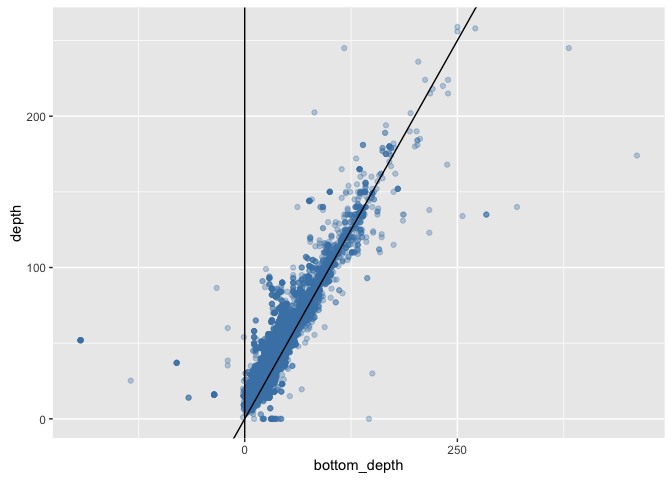
This plot illustrates some of the issues with using an estimate of bottom depth that, while fine resolution (1 minute) for a global dataset, fails to capture small-scale topographic variation resulting in many sample depths being apparently deeper than the bottom depth. This issue is particularly pronounced around coasts, and users may wish to find either a finer scale bathymetric dataset for their region of interest, or else deal with these coastal areas in some other way (e.g. setting all positive values from ETOPO1 to 0, NA, or similar).
It may be useful however to contrast the results for sole (a demersal flatfish) with a known pelagic species from our dataset, such as the moon jelly Aurelia aurita. First, get occurrences:
jelly_occs <- occurrence(scientificname = "Aurelia aurita")
Filter to retain records with valid depths:
jelly_occs <- filter(
  jelly_occs, !is.na(depth) & depth != -9)
nrow(jelly_occs)
## [1] 1897
These records come from all over the world, so obtaining the bathymetry data will take a long time:
bb_jelly <- bbox(SpatialPoints(cbind(jelly_occs$decimalLongitude, jelly_occs$decimalLatitude)))
However, there are a good number of records within the region queried for sole, so we can just consider those for now:
jelly_occs$bottom_depth <- extract(
  sole_bathy_r, dplyr::select(jelly_occs, decimalLongitude, decimalLatitude))
jelly_occs <- filter(jelly_occs, !is.na(bottom_depth))
jelly_occs$bottom_depth <- -jelly_occs$bottom_depth
Now combine this with the sole data:
sole_jelly <- rbind(
  dplyr::select(sole_occs_refined, scientificName, decimalLongitude, decimalLatitude, depth, bottom_depth),
  dplyr::select(jelly_occs, scientificName, decimalLongitude, decimalLatitude, depth, bottom_depth)
)

(sole_v_jelly <- ggplot(sole_jelly, aes(x = bottom_depth, y = depth)) +
  geom_point(aes(colour = scientificName), alpha = 1/3) +
  geom_smooth(aes(colour = scientificName), method = "lm") +
  scale_colour_manual(values = c("darkorange", "steelblue")) +
  geom_abline(slope = 1, intercept = 0) +
  geom_vline(xintercept = 0)
)
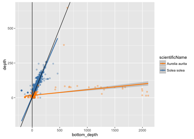
Despite the issues with bottom depth resolution then, this plot nicely shows the contrast between a demersal fish and a pelagic jelly.
This function is a more general implementation of the above code:
get_bottom_depth <- function(occ_dat, bathy_res = 10, bathy_keep = TRUE, bathy_antimerid = FALSE){

  # occ_dat is assumed to be a dataframe as returned from robis::occurrence, including as a minimum the fields:
  # decimalLongitude, decimalLatitude, depth
  # Other arguments are passed to marmap. The default resolution is 10 minutes,
  # defaults for keep and antimeridion are T and F respectively

  # This gets the bathymetry and converts it to a raster
  bb_occs <- bbox(cbind(occ_dat$decimalLongitude, occ_dat$decimalLatitude))
  occs_bathy <- marmap::as.raster(
    getNOAA.bathy(
      lon1 = bb_occs[1, 1], lon2 = bb_occs[1, 2],
      lat1 = bb_occs[2, 1], lat2 = bb_occs[2, 2],
      resolution = bathy_res, keep = bathy_keep, antimeridian = bathy_antimerid
    )
  )

  # This creates the bottom_depth variable in occ dat
  occ_dat$bottom_depth <- -extract(
    occs_bathy, dplyr::select(occ_dat, decimalLongitude, decimalLatitude)
  )

  # record the bathymetry resolution used as an attribute of occ_dat
  attr(occ_dat, "bathymetry_res") <- bathy_res

  # return the occ_dat dataframe with bottom depth added
  return(occ_dat)

}
Quick test on sole data, leaving resolution at 10 minutes for speed:
bathy_test <- get_bottom_depth(sole_occs_refined)
Matching occurrences to temperature in space and time
Matching species occurrences to environmental variables is a very common requirement of macroecological analyses, particularly those considering environmental drivers of species distributions, and how distributions are expected to shift as the climate changes. There are now numerous freely available environmental data layers which differ in the methods employed to generate them, as well as their spatial and temporal resolution. Here we show how to obtain NOAA gridded monthly mean Sea Surface Temperature data and to match occurrence records to temperature in both space and time.
This code is from a package in development with ROpenSci called spenv, see here.
We’ll use slightly modified versions of spenv functions here. First, this function downloads SST data from NOAA. Specifically, it downloads monthly mean data at 1 degree resolution from the Optimum Interpolation Seas Surface Temperature V2 dataset, see here. The data are served as a NetCDF file, but for convenience we transform this into a raster brick - this is essentially a stacked set of global rasters, each layer representing a single month in the time series. The first time you run this the file will be downloaded (takes ~10 seconds). It will then be stored locally for future use:
sst_prep <- function(path = "~/.spenv/noaa_sst") {
  x <- file.path(path, "sst.mnmean.nc")
  if (!file.exists(x)) {
    dir.create(dirname(x), recursive = TRUE, showWarnings = FALSE)
    download.file("ftp://ftp.cdc.noaa.gov/Datasets/noaa.oisst.v2/sst.mnmean.nc", destfile = x)
  }
  raster::brick(x, varname = "sst")
}
So, to get the SST data:
sst_dat <- sst_prep()
View the structure of the data:
sst_dat
## class       : RasterBrick
## dimensions  : 180, 360, 64800, 417  (nrow, ncol, ncell, nlayers)
## resolution  : 1, 1  (x, y)
## extent      : 0, 360, -90, 90  (xmin, xmax, ymin, ymax)
## coord. ref. : +proj=longlat +datum=WGS84 +ellps=WGS84 +towgs84=0,0,0
## data source : /Users/alunjones/.spenv/noaa_sst/sst.mnmean.nc
## names       : X1981.12.01, X1982.01.01, X1982.02.01, X1982.03.01, X1982.04.01, X1982.05.01, X1982.06.01, X1982.07.01, X1982.08.01, X1982.09.01, X1982.10.01, X1982.11.01, X1982.12.01, X1983.01.01, X1983.02.01, ...
## Date        : 1981-12-01, 2016-08-01 (min, max)
## varname     : sst
You can plot a few months too:
plot(sst_dat)
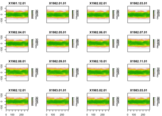
You don’t need to run the above code as it is automatically called from the following functions, but it gives you an idea of the structure of the environmental data:
dim(sst_dat)
## [1] 180 360 417
180 degrees latitude x 360 degrees longitude x 416 months.
This is the wrapper function that takes your input data (x), together with identifiers for latitude, longitude, and date, and gets SST data from the NOAA SST gridded dataset. The origin argument enables conversion between the date formats of the NOAA data and your occurrence data. Note that this data also calculates an adjusted longitude, as occupancy data typically come with longitude in the range -180 (180 West) to +180 (180 East), whereas the NOAA data codes longitude as 0 to 360 degrees (running eastwards from 0 degrees):
sp_extract_gridded_date <- function(x, from = "noaa_sst", latitude = NULL,
                                    longitude = NULL, samp_date = NULL, origin = as.Date("1800-1-1")) {

  x <- spenv_guess_latlondate(x, latitude, longitude, samp_date)
  switch(from,
         noaa_sst = {
           mb <- sst_prep()
           out <- list()
           x <- x[ !is.na(x$date), ]
           x$date <- as.Date(x$date)
           x <- x[x$date >= min(mb@z[["Date"]]), ]
           x$lon_adj <- x$longitude
           x$lon_adj[x$lon_adj < 0] <- x$lon_adj[x$lon_adj < 0] + 360
           for (i in seq_len(NROW(x))) {
             out[[i]] <- get_env_par_space_x_time(mb, x[i, ], origin = origin)
           }
           x$sst <- unlist(out)
           x
         }
  )
}
The following functions are utility functions called by the above function. This takes an occurrence dataset and ensures that latitude, longitude, and date variables are correctly identified and named:
spenv_guess_latlondate <- function(x, lat = NULL, lon = NULL, samp_date = NULL) {
  xnames <- names(x)
  if (is.null(lat) && is.null(lon)) {
    lats <- xnames[grep("^(lat|latitude)$", xnames, ignore.case = TRUE)]
    lngs <- xnames[grep("^(lon|lng|long|longitude)$", xnames, ignore.case = TRUE)]

    if (length(lats) == 1 && length(lngs) == 1) {
      if (length(x) > 2) {
        message("Assuming '", lngs, "' and '", lats,
                "' are longitude and latitude, respectively")
      }
      x <- rename(x, setNames('latitude', eval(lats)))
      x <- rename(x, setNames('longitude', eval(lngs)))
    } else {
      stop("Couldn't infer longitude/latitude columns, please specify with 'lat'/'lon' parameters", call. = FALSE)
    }
  } else {
    message("Using user input '", lon, "' and '", lat,
            "' as longitude and latitude, respectively")
    x <- plyr::rename(x, setNames('latitude', eval(lat)))
    x <- plyr::rename(x, setNames('longitude', eval(lon)))
  }

  if(is.null(samp_date)){
    dates <- xnames[grep("date", xnames, ignore.case = TRUE)]
    if(length(dates) == 1){
      if(length(x) > 2){
        message("Assuming '", dates, "' are sample dates")
      }
      x <- rename(x, setNames('date', eval(dates)))
    } else {
      stop("Couldn't infer sample date column, please specify with 'date' parameter", call. = FALSE)
    }

  } else {
    message("Using user input '", samp_date, "' as sample date")
    x <- plyr::rename(x, setNames('date', eval(samp_date)))
  }

}
This extracts the relevant SST value for a given combination of latitude, longitude, and date. Note that it uses the simple (default) method for extracting values from the SST raster, in the raster::extract call. This means it simply extracts the SST value from the grid square in which each point falls. The bilinear method would interpolate SST values from the nearest 4 squares to a point. Likewise, it is possible to set buffers around each point and perform some function (e.g. mean) on all returned values. For environmental variables with little spatial autocorrelation these methods may be useful.
get_env_par_space_x_time <- function(
  env_dat, occ_dat, origin = as.Date("1800-1-1")){

  # calculate starting julian day for each month in env_dat
  month_intervals <- as.numeric(env_dat@z[["Date"]] - origin)
  # calculate julian day for the focal date (eventDate in occ_dat)
  focal_date <- as.numeric(occ_dat$date - origin)

  # extract environmental variable (SST here) for this point
  as.numeric(raster::extract(
    env_dat,
    cbind(occ_dat$lon_adj, occ_dat$latitude),
    layer = findInterval(focal_date, month_intervals),
    nl = 1
  ))
}
sst_prep <- function(path = "~/.spenv/noaa_sst") {
  x <- file.path(path, "sst.mnmean.nc")
  if (!file.exists(x)) {
    dir.create(dirname(x), recursive = TRUE, showWarnings = FALSE)
    download.file("ftp://ftp.cdc.noaa.gov/Datasets/noaa.oisst.v2/sst.mnmean.nc", destfile = x)
  }
  raster::brick(x, varname = "sst")
}
So, we can add SST data to our sole occurrence data like this. Note that occurrence records with no date of collection information, or which were collected prior to 1981 (when the monthly mean dataset begins) will be stripped from the output. NB - SLOW!!! This takes ~11 minutes:
sole_sst <- sp_extract_gridded_date(x = sole_occs_refined,
                                    latitude = "decimalLatitude", longitude = "decimalLongitude", samp_date = "eventDate")
Check dimensions of returned data:
nrow(sole_sst)
## [1] 57880
sum(sole_occs_refined$yearcollected < 1981)
## [1] 799
Quick plot of derived SST against lat and lon, for each month: first, extract the month from each date using lubridate::month:
sole_sst$month <- month(sole_sst$date)
Now plot occurrences by lon and lat, colour coded by temperature, faceted by month (1 = Jan to 12 = Dec):
(sole_sst_plot <- (ggplot(sole_sst, aes(x = longitude, y = latitude)) +
                     geom_point(aes(colour = sst), alpha = 2/3) +
                     scale_colour_gradient(low = "blue", high = "red") +
                     facet_wrap(~ month))
)
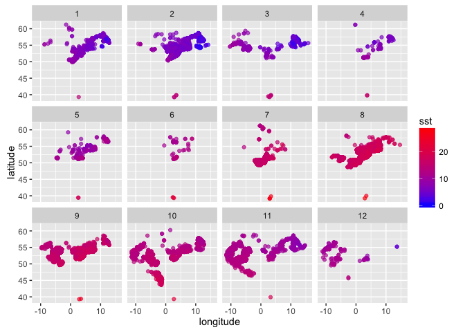
This looks reasonable - SST increases into the summer, and decreases with latitude.
The above matching process could be sped up by only querying for unique combinations of latitude, longitude, and date:
sum(!duplicated(dplyr::select(sole_occs_refined, decimalLatitude, decimalLongitude, eventDate)))
## [1] 9480
Only 9480 unique combinations, of the nearly 60,000 occurrences. Aggregating to the resolution of the environmental dataset will likely reduce this further:
sole_occs_refined$lat <- round(sole_occs_refined$decimalLatitude)
sole_occs_refined$lon <- round(sole_occs_refined$decimalLongitude)
sole_occs_refined$yr_month <- with(sole_occs_refined, paste(yearcollected, month(eventDate), sep = "_"))
sum(!duplicated(dplyr::select(sole_occs_refined, lat, lon, yr_month)))
## [1] 3539
Only 3539.
So: create a dataset with one example occurrence from each combination of lat, lon, and year_month:
sole_temp <- sole_occs_refined[!duplicated(dplyr::select(sole_occs_refined, lat, lon, yr_month)), ]
sole_sst2 <- sp_extract_gridded_date(x = sole_temp,
                                     latitude = "decimalLatitude", longitude = "decimalLongitude", samp_date = "eventDate")
This now runs in ~40s, and results can be joined back into sole_occs_refined, based on a new location_date key:
sole_sst2$loc_date <- with(sole_sst2, paste(lat, lon, yr_month, sep = "_"))
sole_occs_refined$loc_date <- with(sole_occs_refined, paste(lat, lon, yr_month, sep = "_"))
Strip unwanted variables from sole_sst:
sole_sst2 <- dplyr::select(sole_sst2, loc_date, sst)
Perform the join:
sole_occs_refined <- left_join(sole_occs_refined, sole_sst2, by = "loc_date")
And remove intermediate objects:
rm(sole_temp, sole_sst2)
Create month variable, using lubridate::month:
sole_occs_refined$month <- month(sole_occs_refined$eventDate)
Recreate the lat-lon-temp-month plot from above:
sole_sst_plot <- ggplot(subset(
  sole_occs_refined, !is.na(sst)), aes(x = decimalLongitude, y = decimalLatitude)) +
  geom_point(aes(colour = sst), alpha = 2/3) +
  scale_colour_gradient(low = "blue", high = "red") +
  facet_wrap(~ month)
The information collected now enables you to say something about the environmental conditions experienced by a species. For instance, we can show the range of temperatures experienced by sole, for instance getting a Tukey five-number summary (minimum, first quartile, median, third quartile, maximum):
fivenum(sole_occs_refined$sst)
## [1] -0.21 15.08 16.34 17.58 28.41
Or we could look at trends over years in the temperature experienced by sole, within each month:
(sole_sst_trends <- ggplot(subset(sole_occs_refined, !is.na(sst)), aes(x = yearcollected, y = sst)) +
   geom_point(colour = "steelblue", alpha = 1/3) +
   geom_smooth(method = "lm", colour = "darkorange") +
   facet_wrap(~ month)
)
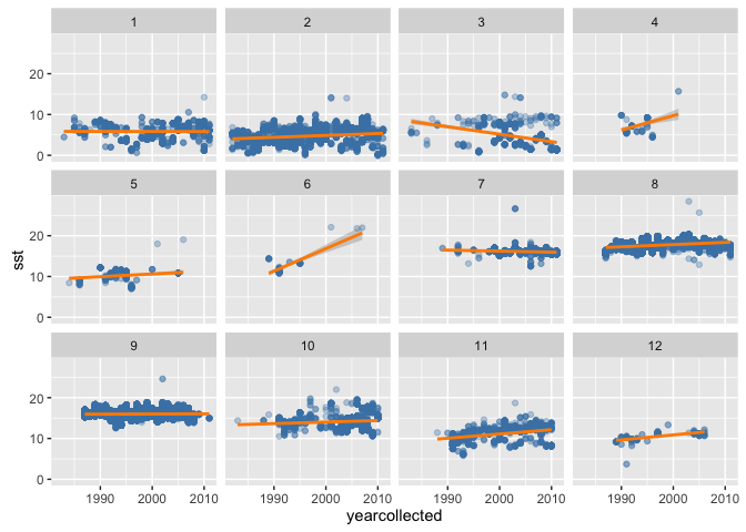
Note: these plots are purely exploratory. As we have already seen, sole are demersal fish and so sea bottom temperature is likely much more important to them than SST. And this plot takes no account of the spatial location of survey points in each year. But it serves to illustrate what is possible.
Matching occurrences to local spatial datasets
The examples above use R to obtain environmental data served over the web. However, there are also numerous spatial datasets that are not easily accessible via web services, that researchers may have either generated themselves, or have obtained from some third party and stored locally. Most frequently these kinds of data are available in some kind of gridded format. Here we provide examples of how to match occurrence records in space only to gridded data freely available from GMED, which we have downloaded to local files ASCII grid files.
Numerous gridded environmental layers are openly available, but they are not always easy to access remotely. For instance, the Global Marine Environment Dataset (GMED) provides time-averaged global layers of a wide range of environmental variables (see Basher, Z., Costello, M. J., Bowden, D. A. 2014. Global Marine Environment Dataset (GMED). World Wide Web electronic publication. Version 1.0 (Rev.01.2014). Accessed at http://gmed.auckland.ac.nz). However these are available as .7z zipped files, a Windows compression format that requires third party software (such as The Unarchiver) to unzip on Mac OSX. The most straightforward approach then is to download and uncompress the files and then load them from a local source. The following example uses the primary productivity data, which is read in as an ascii grid and then converted to a raster. You will need to copy the relevant folder into the data/ folder in your working directory, from here.
env_grid <- raster(read.asciigrid("data/primprod_chla/aq_primprod.asc"))
NB: this is rather a large (68.2MB) object:
object_size(env_grid)
## 68.2 MB
You can plot it to get an idea of the data:
plot(env_grid)
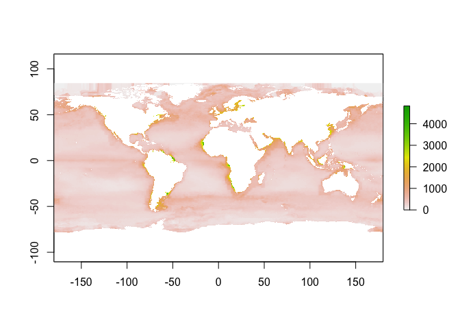
And you can find e.g. the range of values present in the data:
range(env_grid@data@values, na.rm = T)
## [1] 0 4875
hist(env_grid@data@values)
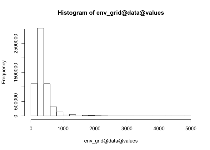
And then you can extract values from environmental grid for occurrence points:
env_occ <- tbl_df(data.frame(extract(
  env_grid, cbind(sole_occs_refined$decimalLongitude, sole_occs_refined$decimalLatitude), cellnumbers = T)))
Or simply add chla values directly back to the original dataframe:
sole_occs_refined$chla <- extract(env_grid,
                                  cbind(sole_occs_refined$decimalLongitude, sole_occs_refined$decimalLatitude))
It is very quick to extract data from a flat raster so there is little to be gained from only querying unique lat-lon combinations here.
Another useful variable available from GMED is bottom temperature (although remember that it is a single long term time averaged layer, so is not directly comparable to the SST data we used above). You will need to add this to your data folder.
env_grid <- raster(read.asciigrid("data/btemp_k/kg_b_temp.asc"))
Again, plot it to get an idea of the data:
plot(env_grid)
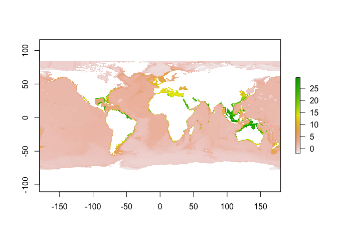
And you can find e.g. the range of values present in the data:
range(env_grid@data@values, na.rm = T)
## [1] -2.08170 29.45666
hist(env_grid@data@values)
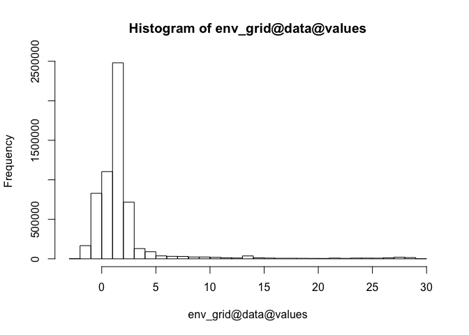
Add to sole_occs_refined:
sole_occs_refined$bottom_temp <- extract(env_grid,
                                         cbind(sole_occs_refined$decimalLongitude, sole_occs_refined$decimalLatitude))
Look at summary:
fivenum(sole_occs_refined$bottom_temp)
## [1] 0.00000 9.94703 10.42849 10.80025 17.90282
Adding geography
All of the examples above have been global in scale, meaning that we have placed no spatial restrictions on the queries to OBIS - we have simply requested all occurrences that have been recorded anywhere on earth. However, we are frequently interested in sub-global analyses, either extracting data for an individual region of interest (such as a specific country’s EEZ), or summarising global data by region (e.g. records per regional sea). Here we show how the Marine Regions database can be accessed programmatically to return OBIS data for a specific named region. We show how to get records for a specific taxon within a named region, or for all taxa within a named region. We also show how to summarise global data at the regional scale, for instance returning number of species or number of OBIS records per region.
Getting occurrence data for a specific region
All of the above work has been based on global data - we have extracted all records from OBIS, regardless of where in the world they come from. Often we have a particular focal region and want to get data only from there. The functions in robis allow such regions to be flexibly specified as a geometry argument in both occurrence and taxa. For instance you can explicitly specify the coordinates of a polygon. Here, we get occurrences of basking shark within the polygon bounded by 0 and -10 degrees longitude and by 50 and 60 degrees latitude:
basking_shark <- occurrence(scientificname = "Cetorhinus maximus",
                            geometry = "POLYGON ((-10 50, -10 60, 0 60, 0 50, -10 50))")
basking_map <- obis_map(basking_shark, map_type = "satellite", map_zoom = 4, plotit = F)
basking_map + geom_rect(aes(xmin = -10, xmax = 0, ymin = 50, ymax = 60), colour = "green", fill = NA)
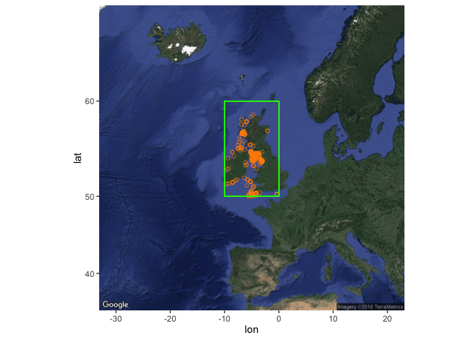
More often you are likely to want to specify some pre-existing region. marineregions.org provides a standard list of marine georeferenced place names and boundaries, including many regional specifications familiar to marine ecologists, such as Exclusive Economic Zones (EEZs), Large Marine Ecosystems (LMEs), IHO Regional Sea Areas, etc. The ROpenSci package mregions (vignette here) provides an interface to this database which allows us to provide specified polygons to OBIS when we query. If you know the name of the region of interest this is straightforward:
uk_eez <- mr_shp("MarineRegions:eez", maxFeatures = NULL, filter = "United Kingdom Exclusive Economic Zone")
We’ll use gSimplify from rgeos to simplify the geometry a bit:
uk_eez_simple <- SpatialPolygonsDataFrame(gSimplify(uk_eez, tol = 0.01, topologyPreserve = TRUE), data = uk_eez@data)
Use the tidy function in broom to convert this to a dataframe for plotting purposes:
uk_eez_df <- tidy(uk_eez_simple)
Re-run the OBIS query:
basking_shark <- occurrence(scientificname = "Cetorhinus maximus",
                            geometry = mr_as_wkt(uk_eez_simple))
Reproduce the map:
basking_map <- obis_map(basking_shark, map_type = "satellite", map_zoom = 4, plotit = F)
Plot the map together with the UK EEZ boundary (I have reduced the line width of bounding polygon here to 0.25):
basking_map +
  geom_polygon(data = uk_eez_df, aes(x = long, y = lat, group = group),
               colour = "green", fill = NA, size = 0.25)
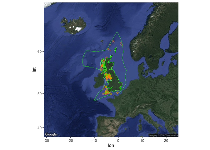
Getting a species list for a specific region
The checklist() function can also take a geometry argument, making it straightforward to get, for instance, summary data for a particular species from within a given region, e.g.:
uk_basking_shark <- checklist(scientificname = "Cetorhinus maximus",
                         geometry = mr_as_wkt(uk_eez_simple))
Perhaps more useful is to get a taxon list for a region. The UK has an unusually large density of OBIS records so for a faster query we’ll use a different EEZ, here Albania. We’ll use the geo_json format instead of shape files here:
geo <- mr_geojson(key = "MarineRegions:eez", filter = "Albanian Exclusive Economic Zone", maxFeatures = NULL)
alb_eez <- mr_as_wkt(geo, fmt = 5)
alb_taxa <- tbl_df(checklist(geometry = alb_eez))
This returns a list of taxa, of various ranks. If we wanted a species list, we can get that easily:
alb_species <- filter(alb_taxa, rank_name == "Species")
This gives us a list of species recorded within the Albanian EEZ, together with useful taxonomic data and summary info as described in our first demonstration of the checklist() function above.
Finding appropriate region names
The above examples assume that you already know the exact name of the region that interests you, but this is not always the case. You can of course check on marineregions.org, but mregions provides a number of functions to help you without having to leave R.
You can get a list of place types - different categories of regions:
reg_types <- mr_place_types()
You can see all of the types like this:
sort(reg_types$type)
##  [1] "Abyssal Plain"       "Abyssal Provinces"   "Anchorage"
##  [4] "Apron"               "Aquifer"             "Archipelagic waters"
##  [7] "Archipelago"         "Arctic Marine Area"  "Area"
## [10] "Arm"
##  [ reached getOption("max.print") -- omitted 291 entries ]
EEZ is there, also things like FAO divisions, ICES Areas, Marine Ecoregions of the World, etc. To find region types matching a string of interest, try:
reg_types[grepl("IHO", reg_types[, 1], ignore.case = TRUE), ]
##             type description
## 236 IHO Sea Area        <NA>
reg_types[grepl("ICES", reg_types[, 1], ignore.case = TRUE), ]
##                            type
## 216              ICES Ecoregion
## 286                  ICES Areas
## 287 ICES Statistical Rectangles
##                                                                                                                                                                                                                                                 description
## 216          ICES EcoRegions are largescale management units that are used in ICES advisory reports and were first referenced in the ACFM/ACME report of 2004 (now ACOM) [http://www.ices.dk/datacentre/updates/DC_update.htm?WT.mc_id=DCeNews_March_2009].
## 286 The ICES Statistical Areas delineates the divisions and subdivisions of FAO Major Fishing area 27.\r\nThe ICES Statistical Areas are used as bounding areas for calculation of fish statistics, e.g. catch per unit effort (CPUE) and stock estimates.
## 287                                                                                                                                                                                                                                                    <NA>
Note this is case insensitive:
reg_types[grepl("eez", reg_types[, 1], ignore.case = TRUE), ]
##                   type
## 64                 EEZ
## 297 Joint regime (EEZ)
##                                                                                                                                                                                                                                                                                                                                        description
## 64  In international maritime law, an exclusive economic zone (EEZ) is a seazone extending from a state's coast over which the state has special rights over the exploration and use of marine resources. Generally a state's EEZ extends 200 nautical miles out from its coast, except where resulting points would be closer to another country.
## 297                                                                                                                                                        A geographical area delimited by agreement between two or more countries where with specific arrangements in relation to the exploration and exploitation of natural marine resources.
Once you have the name of the type of region you want, you can get a list of all named regions under that scheme using, for example (and note this is case sensitive):
eez_ids <- tbl_df(mr_records_by_type(type = "EEZ"))
iho_ids <- tbl_df(mr_records_by_type(type = "IHO Sea Area"))
An issue here is that you are limited to returning only the first 100 features; for EEZs we know there are more than that. The following is a workaround:
all_mr_records_by_type <- function(mr_type){

  mr_ids <- mr_records_by_type(type = mr_type)
  if(nrow(mr_ids) == 100){
    new_q <- TRUE
    while(new_q == T){
      next_recs <- mr_records_by_type(type = mr_type, offset = nrow(mr_ids))
      if(length(next_recs) == 0){
        new_q <- FALSE
      } else {
        mr_ids <- rbind(mr_ids, next_recs)
        if(nrow(eez_ids) %% 100 != 0){new_q <- FALSE}
      }
    }
  }
  return(tbl_df(mr_ids))

}

eez_ids <- all_mr_records_by_type(mr_type = "EEZ")
You can now find preferred names for all regions within the scheme (here, all individual EEZs) as:
sort(eez_ids$preferredGazetteerName)
##  [1] "Albanian Exclusive Economic Zone"
##  [2] "Algerian Exclusive Economic Zone"
##  [3] "American Samoa Exclusive Economic Zone"
##  [4] "Amsterdam Island & St. Paul Island Exclusive Economic Zone"
##  [5] "Angolan Exclusive Economic Zone"
##  [6] "Anguilla Exclusive Economic Zone"
##  [7] "Antarctic 200NM zone beyond the coastline"
##  [8] "Antigua and Barbuda Exclusive Economic Zone"
##  [9] "Area of overlap between Australian Seabed Jurisdiction and Indonesian Exclusive Economic Zone Jurisdiction"
## [10] "Argentinean Exclusive Economic Zone"
##  [ reached getOption("max.print") -- omitted 241 entries ]
And you can then feed this into the above, e.g.:
tax_list <- tbl_df(checklist(geometry = mr_as_wkt(mr_geojson(key = "MarineRegions:eez", filter = eez_ids$preferredGazetteerName[1], maxFeatures = NULL), fmt = 5)))
Add a region_name attribute for convenience:
attr(tax_list, "region_name") <- eez_ids$preferredGazetteerName[1]
Check it:
attr(tax_list, "region_name")
## [1] "Belgian Exclusive Economic Zone"
Summarising global data by region
Sometimes you may want summarise your occurrence data by region. We will do that for the occurrence data we generated above for full sorby collection list (allspp_obis), using IHO regional seas as our regions dataset.
We can download shape files for all regions within this scheme, but to do this we need to get the appropriate key for our scheme, which is slightly different from the type identified above. We can get a list of all scheme names using:
rnames <- mr_names()
And we can then search within this for anything containing IHO (case sensitive):
mr_names_search(rnames, "IHO")
## # A tibble: 5 × 4
##                                   name
##                                  <chr>
## 1                    MarineRegions:iho
## 2 MarineRegions:iho_quadrants_20150810
## 3                     World:iosregions
## 4       MarineRegions:eez_iho_union_v2
## 5                   Belgium:vl_venivon
## # ... with 3 more variables: title <chr>, name_first <chr>,
## #   name_second <chr>
We want the Marine Regions version of the IHO regions, "MarineRegions:iho", which we can then use like this:
iho_regions <- mr_shp(key = "MarineRegions:iho", maxFeatures = 1000)
maxFeatures is the maximum number of features to download, with a default of 50. If you think your scheme may have more than 50 component features, but you’re not sure how many, set it to something arbitrarily large (e.g. here we have used 1000).
Also note other useful region schemas such as World:grid5deg - a 5 degree grid of the world:
wgrid <- mr_shp(key = "World:grid5deg", maxFeatures = 1000)
#plot(wgrid)
This can be really useful for summarising occurrence data. You can browse through all region schemas using e.g.:
sort(rnames$name)
The following function allows you to plot these regions - it is not very polished but serves to show more or less where the regions are, and to identify any issues there may be. It takes a shape file similar to the one just generated as iho_regions, or a dataframe produced by applying the function broom::tidy to such a spatial polygons dataframe, and adds the regions to a world map. It will either colour the regions and provide a key (poly_fill = TRUE) or just plot their outlines (poly_fill = FALSE). fill_by allows polygons to be filled according to an additional variable, and is explained below.
region_map <- function(regions, poly_fill = TRUE, fill_by = NULL, plotit = TRUE){

  # get the base map
  base_map <- map_data("world")
  region_map <- ggplot(base_map, aes(x=long, y=lat)) +
    geom_polygon(aes(group=group)) +
    scale_y_continuous(breaks = (-2:2) * 30) +
    scale_x_continuous(breaks = (-4:4) * 45) +
    theme(panel.background = element_rect(fill = NA)) +
    coord_equal()

  # process the regions data into a dataframe, if necessary; add region names, and plot as polygons
  if(class(regions) == "SpatialPolygonsDataFrame"){
    regions@data$id_new <- rownames(regions@data)
    # Create the dataframe
    regions_df <- tidy(regions)
    # Add missing info - specifically region name
    regions_df <- left_join(regions_df, regions@data, by = c("id" = "id_new"))

  } else {
    regions_df <- regions
  }

  if(is.null(fill_by)){
    if(poly_fill == TRUE){
      region_map <- region_map +
        geom_polygon(data = regions_df,
                     aes(x = long, y = lat, group = group, fill = name), alpha = 1/3) +
        theme(legend.position = "top") +
        theme(legend.text = element_text(size = 4)) +
        theme(legend.title = element_blank())
    } else {
      region_map <- region_map +
        geom_polygon(data = regions_df,
                     aes(x = long, y = lat, group = group), fill = NA, colour = "green")
    }
  } else {
    id_fill <- which(names(regions_df) %in% fill_by)
    names(regions_df)[id_fill] <- "fill_var"
    region_map <- region_map +
      geom_polygon(data = regions_df,
                   aes(x = long, y = lat, group = group, fill = fill_var)) +
      scale_fill_gradient(name = fill_by) +
      theme(legend.position = "top")
  }

  if(plotit == TRUE){print(region_map)}
}
As an example:
region_map(regions = iho_regions)
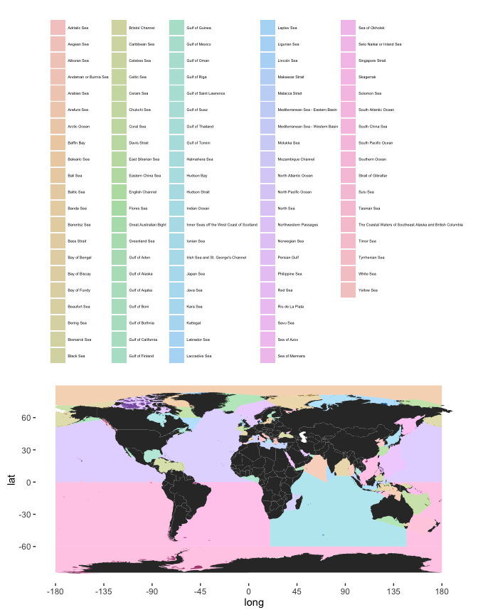
Just plot region outlines:
region_map(regions = iho_regions, poly_fill = FALSE)
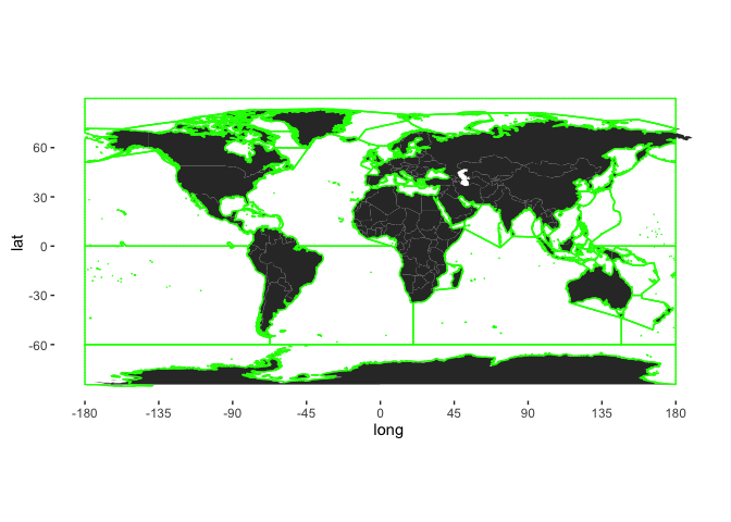
To identify the region in which each occurrence point in your occurrence dataset occurs, we need to do a little processing. First, we need to transform the occurrences into a SpatialPointsDataFrame. This has to have the same projection as the regions shape file - for convenience here we will impose that condition, but for serious geospatial analyses more attention should be paid to projections.
For the purposes of illustration we will work on a sample of 10000 occurrence points:
samp_obis <- sample_n(allspp_obis, 10000)
Create the spatial dataframe:
samp_obis_spat <- SpatialPointsDataFrame(
  coords = cbind(samp_obis$decimalLongitude, samp_obis$decimalLatitude),
  data = samp_obis, proj4string = crs(iho_regions))
Now for each point we can get the ID of the region in which it occurs:
allspp_obis_regionid <- over(samp_obis_spat, iho_regions)
head(allspp_obis_regionid)
##              name id mrgid
## 125747  North Sea  4  2350
## 675224   Kattegat  2  2374
## 942273  Skagerrak  3  2379
## 917531  Skagerrak  3  2379
## 1196617 North Sea  4  2350
## 1081563 North Sea  4  2350
This can now be added back into our original dataframe:
samp_obis$iho_region <- allspp_obis_regionid$name
head(samp_obis)
##                scientificName decimalLongitude decimalLatitude depth
## 125747      Lanice conchilega        -2.966073        56.09899    NA
## 675224   Merlangius merlangus        11.866700        56.60000    31
## 942273  Pleuronectes platessa        10.732500        58.08380   227
## 917531  Pleuronectes platessa         9.166700        57.35000    20
## 1196617           Solea solea         2.715300        51.45780    29
## 1081563 Pleuronectes platessa         0.502500        57.24510    -9
##         yearcollected iho_region
## 125747           1993  North Sea
## 675224           1995   Kattegat
## 942273           2008  Skagerrak
## 917531           2002  Skagerrak
## 1196617          2009  North Sea
## 1081563          2009  North Sea
And region-level summaries can be obtained, for instance by grouping the data by iho_region:
by_region <- group_by(samp_obis, iho_region)
This then gives total number of OBIS records, and number of species, for each iho_region:
iho_summaries <- dplyr::summarise(by_region,
                                  n_obis_records = n(),
                                  n_species = n_distinct(scientificName)
)
By adding in more taxonomic information (or returning more of it from the original OBIS query), it would be possible to get higher taxon summaries too.
To put these summaries on a map, first convert the iho_regions data into a dataframe. This requires a little fiddling to ensure IDs match properly:
iho_regions@data$id_new <- rownames(iho_regions@data)
Create the dataframe:
iho_regions_df <- tidy(iho_regions)
And add missing info - specifically region name:
iho_regions_df <- left_join(iho_regions_df, iho_regions@data, by = c("id" = "id_new"))
head(iho_regions_df)
##        long      lat order  hole piece group id
## 1 -6.496945 58.08749     1 FALSE     1   0.1  0
## 2 -6.513241 58.08596     2 FALSE     1   0.1  0
## 3 -6.529536 58.08444     3 FALSE     1   0.1  0
## 4 -6.545832 58.08291     4 FALSE     1   0.1  0
## 5 -6.562127 58.08138     5 FALSE     1   0.1  0
## 6 -6.578423 58.07985     6 FALSE     1   0.1  0
##                                        name id.y mrgid
## 1 Inner Seas off the West Coast of Scotland   18  4283
## 2 Inner Seas off the West Coast of Scotland   18  4283
## 3 Inner Seas off the West Coast of Scotland   18  4283
## 4 Inner Seas off the West Coast of Scotland   18  4283
## 5 Inner Seas off the West Coast of Scotland   18  4283
## 6 Inner Seas off the West Coast of Scotland   18  4283
Now add the summary data created above:
iho_regions_df <- left_join(iho_regions_df, iho_summaries, by = c("name" = "iho_region"))
This can now be plotted using the region_map function from above, now feeding in a fill_by argument:
region_map(iho_regions_df, fill_by = "n_obis_records")
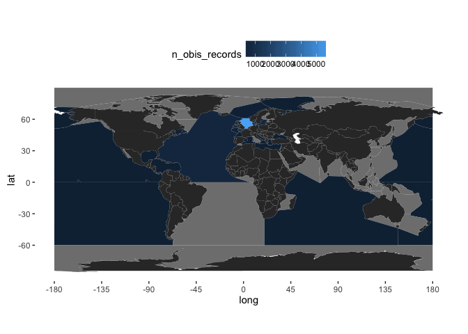
Note that for our rather small sample, there will probably be a number of regions with no OBIS records or species here. But the principle is sound.
At present, if you wanted to plot, say, log-transformed number of records, you’d need to create a new variable in the dataframe, e.g.:
iho_regions_df$log_OBIS_records <- log10(iho_regions_df$n_obis_records)
region_map(iho_regions_df, fill_by = "log_OBIS_records")
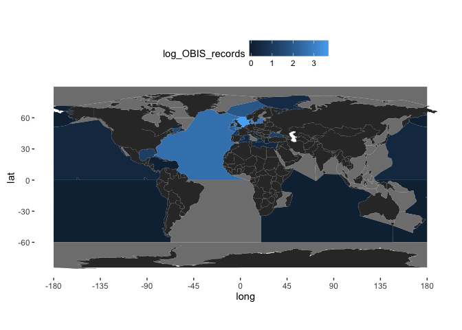
Combining Regional and Environmental Data
We next show how regional and environmental data can be combined to return records from a particular environmental subset of a region. For instance, you might be interested only in parts of the North Atlantic that are <500m deep, or you might want to focus on regions of the global oceans with an average bottom temperature above some minimum value. Once you have defined your area of interest based on such environmental constraints, you can then use the resulting polygon to return OBIS records.
Here we will take a large region, the North Atlantic Ocean IHO Sea Area. Get the North Atlantic polygon:
n_atlantic <- subset(iho_regions, name == "North Atlantic Ocean")
Have a look at it:
region_map(n_atlantic)
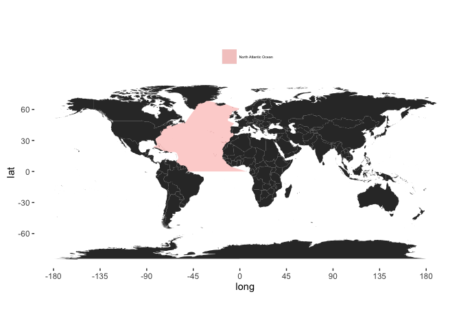
Get its extent:
region_bb <- bbox(n_atlantic)
Use marmap again to get bathymetry for this region - here using 10 min resolution for speed:
region_bathy <- marmap::as.raster(
  getNOAA.bathy(
    lon1 = region_bb[1, 1], lon2 = region_bb[1, 2],
    lat1 = region_bb[2, 1], lat2 = region_bb[2, 2],
    resolution = 10, keep = TRUE, antimeridian = FALSE
  )
)
Quick look:
plot(region_bathy)
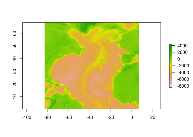
Now, mask this bathymetry raster using the region polygon:
region_bathy <- mask(region_bathy, n_atlantic)
plot(region_bathy)
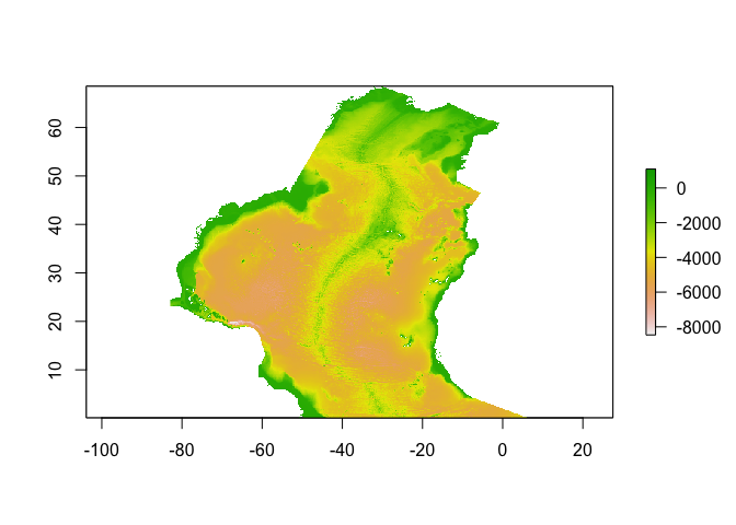
You can extract useful info here using cellStats, for instance the range of depths in your region:
cellStats(region_bathy, stat = range)
## [1] -8467 1089
And the number of ‘positive depths’ (indicating land):
cellStats(region_bathy > 0, stat = sum)
## [1] 503
NB: the max value here is +1089, and 503 grid squares have values > 0, presumably due to the resolution we used for bathymetry overlapping coastal areas, incorporating oceanic islands, etc.
You can find the number of cells meeting some set of criteria, e.g. lying in a particular depth range. First, set your criteria - here, cells between 0 and 500m deep:
mindepth <- 0
maxdepth <- -500
How many cells match this?
cellStats(region_bathy <= mindepth & region_bathy >= maxdepth, stat = sum)
## [1] 10362
10362 cells are in this range. To get the cell IDs (actually, this finds cells that do NOT match criteria, so they can be changed to NA):
id_out_of_depth <- which(values(region_bathy) < maxdepth | values(region_bathy) > mindepth)
region_bathy_cut <- region_bathy
region_bathy_cut[id_out_of_depth] <- NA
This now identifies all cells within the North Atlantic less then 500m deep:
plot(region_bathy_cut)
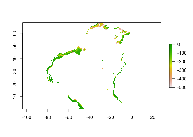
To make matching to a new data source (e.g. occurrence data) easier, here is an alternative approach which creates a polygon out of cells matching the criteria. First, extract the part of the grid that matches your criteria - NB: this can be a bit slow:
region_bathy_poly <- rasterToPolygons(region_bathy, fun = function(x){x <= mindepth & x >= maxdepth})
Plot if you like but this will take a long time to render when the number of polygons is large; much quicker to simplify by combining subgeometries using rgeos::gUnaryUnion:
region_bathy_poly <- gUnaryUnion(region_bathy_poly)
plot(region_bathy_poly)
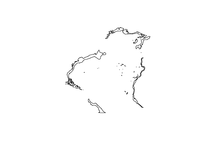
You now have a spatialPolygon outlining all suitable depths within your region, which you can use to extract values from another environmental raster - trivially (but again, rather slowly), for depth:
value_within_region <- extract(region_bathy, y = region_bathy_poly, df = T)
head(value_within_region)
##   ID layer
## 1  1   -18
## 2  1   -21
## 3  1   -84
## 4  1  -185
## 5  1  -314
## 6  1  -214
names(value_within_region)[2] <- "env_variable"
To check - all values here should be between mindepth and maxdepth:
range(value_within_region$env_variable)
## [1] -500 0
Supposing you used a useful environmental variable in place of region_bathy here (e.g. Temperature) you can now easily get mean, range, sd, etc. NB: the environmental variable does not need to be the exact shape of your region - a global grid would work, e.g. the bottom temperature grid from GMED we used earlier:
bt_within_region <- extract(env_grid, y = region_bathy_poly, df = T)
head(bt_within_region)
##   ID data.btemp_k.kg_b_temp.asc
## 1  1                   2.275093
## 2  1                   2.269944
## 3  1                         NA
## 4  1                         NA
## 5  1                   2.250614
## 6  1                   1.911228
fivenum(bt_within_region[,2])
## [1] -2.081700 4.552719 7.994298 14.232640 28.531600
Of course you can also use this method of finding ‘environmentally suitable areas’ directly on gridded data (in raster format), e.g. to find those areas globally with a bottom temperature >15 degrees:
min_bt_poly <- rasterToPolygons(env_grid, fun = function(x){x >= 15})
min_bt_poly <- gUnaryUnion(min_bt_poly)
plot(min_bt_poly)
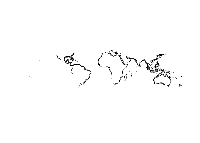
Polygons defined in this way (providing they are not too complex) can then be fed into OBIS queries. (For more complex polygons it is probably easier to query OBIS with a simple bounding box and then crop the returned occurrences to your polygon within R). For instance, to get a list of fish species occurring in water of 1000m or more depth in the North Atlantic (note, the depth constraint here is bottom depth, not sample depth). These queries can take a long time to run if polygons are large and/or complex, or if the taxonomic group queried is speciose. The mammal query here takes around 1.5 minutes for me to run:
region_bathy_poly <- rasterToPolygons(region_bathy, fun = function(x){x < -1000})
region_bathy_poly <- gUnaryUnion(region_bathy_poly)
plot(region_bathy_poly)
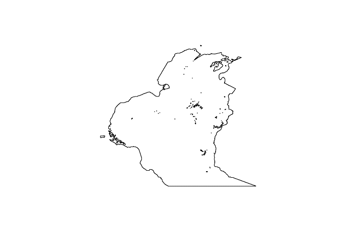
deep_mammals <- checklist(scientificname = "Mammalia", geometry = writeWKT(region_bathy_poly))
deep_mammals <- tbl_df(subset(deep_mammals, rank_name == "Species"))
deep_mammals
## # A tibble: 43 × 17
##        id valid_id parent_id rank_name                      tname
## *   <int>    <int>     <int>     <chr>                      <chr>
## 1  409229   409229    769778   Species         Balaena mysticetus
## 2  409235   409235    739484   Species      Balaenoptera borealis
## 3  409238   409238    739484   Species      Balaenoptera musculus
## 4  409240   409240    739484   Species      Balaenoptera physalus
## 5  432569   432569    769784   Species      Delphinapterus leucas
## 6  432575   432575    432573   Species          Delphinus delphis
## 7  443716   443716    443715   Species           Feresa attenuata
## 8  446724   446724    629011   Species Globicephala macrorhynchus
## 9  446726   446726    629011   Species         Globicephala melas
## 10 448800   448800    448799   Species            Grampus griseus
## # ... with 33 more rows, and 12 more variables: tauthor <chr>,
## #   worms_id <int>, redlist <lgl>, status <chr>, records <int>,
## #   datasets <int>, phylum <chr>, order <chr>, family <chr>, genus <chr>,
## #   species <chr>, class <chr>
So, 43 species of marine mammal have been recorded in deep water in the North Atlantic.
Coda
Nothing in biodiversity research stands still. New data sources are continually coming online. For instance, WoRMS has now started to integrate information on the biological traits of marine organisms into its taxonomic database, in its new traits site. These should be available via web services soon, and we aim to show how to integrate these kinds of data into the above work flows. And just to prove that a job is never done, whilst writing this the displays in Animal & Plant Science have been undergoing work, and the spectacular new version of the Sorby Collection has just been unveiled. So - more species, more data, more work. Onwards!

This post was supported by the DIPS-4-Ocean Assessments project, funded through the Flanders UNESCO Science Trust Fund, which aims to develop biodiversity indices based on OBIS to support global assessments on the state of the marine environment.
![]()